Normal (Gaussian) Distribution

The normal (or Gaussian) distribution is a two-parameter continuous probability distribution. The table below summarizes some important aspects of the distribution.

Notation	\(X \sim \mathcal{N}(\mu, \sigma)\)
Parameters	\(\mu \in \mathbb{R}\) (mean, or location parameter)
	\(\sigma > 0\) (standard deviation, or scale parameter)
Support	\(\mathcal{D}_X = (-\infty, \infty)\)
PDF	\(f_X (x; \mu, \sigma) = \frac{1}{\sigma \sqrt{2 \pi}} \exp \left[ -\frac{1}{2} {\left(\frac{x - \mu}{\sigma}\right)}^2 \right] \)
CDF	\(F_X (x; \mu, \sigma) = \frac{1}{2} \left[ 1 + \mathrm{erf}\left( \frac{x - \mu}{\sigma \sqrt{2}}\right) \right]\)
ICDF	\(F^{-1}_X (x; \mu, \sigma) = \mu + \sqrt{2} \, \sigma \, \mathrm{erf}^{-1}(2 x - 1)\)

error function (\(\mathrm{erf}\))

The error function appearing in the formula for CDF above is defined as

\[ \mathrm{erf}(x) = \frac{2}{\sqrt{\pi}} \int_0^x e^{-t^2} dt \]

and whose domain is \([-1, 1]\).

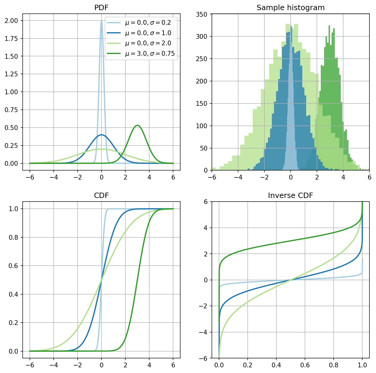
The plots of probability density functions (PDFs), sample histogram (of \(5'000\) points), cumulative distribution functions (CDFs), and inverse cumulative distribution functions (ICDFs) for different parameter values are shown below.

Standard normal distribution

A normal distribution of particular importance is the standard normal distribution whose mean and standard deviation are \(0.0\) and \(1.0\), respectively. The PDF and CDF of the standard normal distribution are usually denoted as \(\phi\) and \(\Phi\). That is

\[ \phi(x) = \frac{1}{\sqrt{2 \pi}} \exp{\left[ - \frac{x^2}{2} \right]}, \]

\[ \Phi(x) = \frac{1}{2} \left[ 1 + \mathrm{erf}\left( \frac{x}{\sqrt{2}}\right) \right], \]

and

\[ \Phi^{-1}(x) = \sqrt{2} \mathrm{erf}(2 x - 1). \]

Any normally distributed random variable can be cast as a transformation of the standard normal distribution. Specifically, the random variable \(X \sim \mathcal{N}(\mu, \sigma)\) can be written as

\[ X = \mu + \sigma Z, \]

where \(Z \sim \mathcal{N}(0, 1)\).