Damped Oscillator Model#
import numpy as np
import matplotlib.pyplot as plt
import uqtestfuns as uqtf
The damped oscillator model is a seven-dimensional scalar-valued function. The model was first proposed in [IK85] and used in the context of reliability analysis in [DKDS91, Dub11].
Note
The reliability analysis variant differs from this base model. Used in the context of reliability analysis, the model also includes additional parameters of a capacity factor and load such that the performance function can be computed. This base model only computes the relative displacement of the spring.
Test function instance#
To create a default instance of the damped oscillator model:
my_testfun = uqtf.DampedOscillator()
Check if it has been correctly instantiated:
print(my_testfun)
Function ID      : DampedOscillator
Input Dimension  : 7 (fixed)
Output Dimension : 1
Parameterized    : False
Description      : Damped oscillator model from Igusa and Der Kiureghian (1985)
Applications     : metamodeling, sensitivity
Description#
The damped oscillator model is based on a two degree-of-freedom primary-secondary mechanical system characterized by two masses, two springs, and the corresponding damping ratios. Originally, the model computes the mean-square relative displacement of the secondary spring under a white noise base acceleration using the following analytical formula[1]:
where \(\boldsymbol{x} = \{ M_p, M_s, K_p, K_s, \zeta_p, \zeta_s, S_0 \}\) is the seven-dimensional vector of input variables further defined below.
Note
In UQTestFuns, this original output is square-rooted to get the relative displacement
Probabilistic input#
Based on [DKDS91], the probabilistic input model for the damped oscillator model consists of seven independent random variables with marginal distributions shown in the table below.
Show code cell source
print(my_testfun.prob_input)
Function ID     : DampedOscillator
Input ID        : DerKiureghian1991
Input Dimension : 7
Description     : Probabilistic input model for the Damped Oscillator model
                  from Der Kiureghian and De Stefano (1991).
Marginals       :

 No.    Name    Distribution          Parameters                   Description
-----  ------  --------------  -------------------------  -----------------------------
  1      Mp      lognormal      [0.40048994 0.09975135]           Primary mass
  2      Ms      lognormal     [-4.61014535  0.09975135]         Secondary mass
  3      Kp      lognormal     [-0.01961036  0.1980422 ]    Primary spring stiffness
  4      Ks      lognormal     [-4.62478054  0.1980422 ]   Secondary spring stiffness
  5    Zeta_p    lognormal     [-3.06994228  0.38525317]      Primary damping ratio
  6    Zeta_s    lognormal     [-4.02359478  0.47238073]     Secondary damping ratio
  7      S0      lognormal      [4.60019502 0.09975135]   White noise base acceleration

Copulas         : Independence
Reference results#
This section provides several reference results of typical UQ analyses involving the test function.
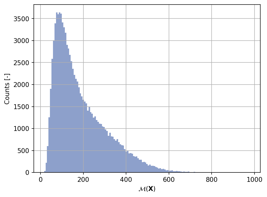
Sample histogram#
Shown below is the histogram of the output based on \(100'000\) random points:
Show code cell source
np.random.seed(42)
xx_test = my_testfun.prob_input.get_sample(100000)
yy_test = my_testfun(xx_test)

plt.hist(yy_test, bins="auto", color="#8da0cb");
plt.grid();
plt.ylabel("Counts [-]");
plt.xlabel("$\mathcal{M}(\mathbf{X})$");
plt.gcf().set_dpi(150);
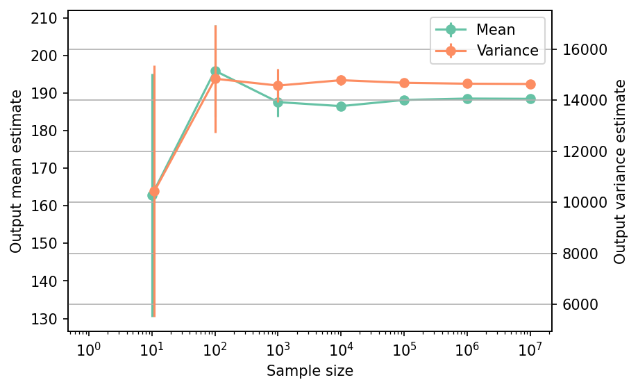
Moments estimation#
Shown below is the convergence of a direct Monte-Carlo estimation of the output mean and variance with increasing sample sizes.
Show code cell source
# --- Compute the mean and variance estimate
np.random.seed(42)
sample_sizes = np.array([1e1, 1e2, 1e3, 1e4, 1e5, 1e6, 1e7], dtype=int)
mean_estimates = np.empty(len(sample_sizes))
var_estimates = np.empty(len(sample_sizes))

for i, sample_size in enumerate(sample_sizes):
    xx_test = my_testfun.prob_input.get_sample(sample_size)
    yy_test = my_testfun(xx_test)
    mean_estimates[i] = np.mean(yy_test)
    var_estimates[i] = np.var(yy_test)

# --- Compute the error associated with the estimates
mean_estimates_errors = np.sqrt(var_estimates) / np.sqrt(np.array(sample_sizes))
var_estimates_errors = var_estimates * np.sqrt(2 / (np.array(sample_sizes) - 1))

# --- Do the plot
fig, ax_1 = plt.subplots(figsize=(6,4))

ax_1.errorbar(
    sample_sizes,
    mean_estimates,
    yerr=mean_estimates_errors,
    marker="o",
    color="#66c2a5",
    label="Mean",
)
ax_1.set_xlabel("Sample size")
ax_1.set_ylabel("Output mean estimate")
ax_1.set_xscale("log");
ax_2 = ax_1.twinx()
ax_2.errorbar(
    sample_sizes + 1,
    var_estimates,
    yerr=var_estimates_errors,
    marker="o",
    color="#fc8d62",
    label="Variance",
)
ax_2.set_ylabel("Output variance estimate")

# Add the two plots together to have a common legend
ln_1, labels_1 = ax_1.get_legend_handles_labels()
ln_2, labels_2 = ax_2.get_legend_handles_labels()
ax_2.legend(ln_1 + ln_2, labels_1 + labels_2, loc=0)

plt.grid()
fig.set_dpi(150)
The tabulated results for each sample size is shown below.
Show code cell source
from tabulate import tabulate

# --- Compile data row-wise
outputs = []
for (
    sample_size,
    mean_estimate,
    mean_estimate_error,
    var_estimate,
    var_estimate_error,
) in zip(
    sample_sizes,
    mean_estimates,
    mean_estimates_errors,
    var_estimates,
    var_estimates_errors,
):
    outputs += [
        [
            sample_size,
            mean_estimate,
            mean_estimate_error,
            var_estimate,
            var_estimate_error,
            "Monte-Carlo",
        ],
    ]

header_names = [
    "Sample size",
    "Mean",
    "Mean error",
    "Variance",
    "Variance error",
    "Remark",
]

tabulate(
    outputs,
    headers=header_names,
    floatfmt=(".1e", ".4e", ".4e", ".4e", ".4e", "s"),
    tablefmt="html",
    stralign="center",
    numalign="center",
)
| Sample size | Mean | Mean error | Variance | Variance error | Remark |
|---|---|---|---|---|---|
| 1.0e+01 | 1.6280e+02 | 3.2313e+01 | 1.0441e+04 | 4.9222e+03 | Monte-Carlo |
| 1.0e+02 | 1.9596e+02 | 1.2183e+01 | 1.4842e+04 | 2.1096e+03 | Monte-Carlo |
| 1.0e+03 | 1.8760e+02 | 3.8178e+00 | 1.4576e+04 | 6.5217e+02 | Monte-Carlo |
| 1.0e+04 | 1.8653e+02 | 1.2160e+00 | 1.4787e+04 | 2.0912e+02 | Monte-Carlo |
| 1.0e+05 | 1.8817e+02 | 3.8319e-01 | 1.4684e+04 | 6.5668e+01 | Monte-Carlo |
| 1.0e+06 | 1.8854e+02 | 1.2103e-01 | 1.4649e+04 | 2.0716e+01 | Monte-Carlo |
| 1.0e+07 | 1.8847e+02 | 3.8260e-02 | 1.4638e+04 | 6.5463e+00 | Monte-Carlo |
References#
Takeru Igusa and Armen Der Kiureghian. Dynamic characterization of two-degree-of-freedom equipment-structure systems. Journal of Engineering Mechanics, 111(1):1–19, 1985. doi:10.1061/(asce)0733-9399(1985)111:1(1).
Armen Der Kiureghian and Mario De Stefano. Efficient algorithm for second-order reliability analysis. Journal of Engineering Mechanics, 117(12):2904–2923, 1991. doi:10.1061/(asce)0733-9399(1991)117:12(2904).