OTL Circuit Function

import numpy as np
import matplotlib.pyplot as plt
import uqtestfuns as uqtf

The OTL circuit test function is a six-dimensional scalar-valued function. The function has been used as a test function in metamodeling exercises [BAS07] and sensitivity analysis [Moo10]. In [Moo10], a 20-dimensional variant was used for sensitivity analysis by introducing 14 additional inert input variables.

Test function instance

To create a default instance of the OTL circuit test function:

my_testfun = uqtf.OTLCircuit()

Check if it has been correctly instantiated:

print(my_testfun)

Function ID      : OTLCircuit
Input Dimension  : 6 (fixed)
Output Dimension : 1
Parameterized    : False
Description      : Output transformerless (OTL) circuit model from Ben-Ari and Steinberg (2007)
Applications     : metamodeling, sensitivity

Description

The OTL circuit function computes the mid-point voltage of an output transformerless (OTL) push-pull circuit using the following analytical formula:

\[\begin{split} \begin{align} \mathcal{M}(\boldsymbol{x}) & = \frac{(V_{b1} + 0.74) \beta (R_{c2} + 9)}{\beta (R_{c2} + 9) + R_f} + \frac{11.35 R_f}{\beta (R_{c2} + 9) + R_f} + \frac{0.74 R_f \beta (R_{c2} + 9)}{(\beta (R_{c2} + 9) + R_f) R_{c1}}, \\ V_{b1} & = \frac{12 R_{b2}}{R_{b1} + R_{b2}}, \\ \end{align} \end{split}\]

where \(\boldsymbol{x} = \{ R_{b1}, R_{b2}, R_f, R_{c1}, R_{c2}, \beta \}\) is the six-dimensional vector of input variables further defined below.

Probabilistic input

Two probabilistic input model specifications for the OTL circuit function are available as shown in the table below.

No.	Keyword	Source
1.	BenAri2007 (default)	[BAS07]
2.	Moon2010	[Moo10]

The default selection, based on [BAS07], contains six input variables given as independent uniform random variables with specified ranges shown in the table below.

Show code cell source Hide code cell source

print(my_testfun.prob_input)

Function ID     : OTLCircuit
Input ID        : BenAri2007
Input Dimension : 6
Description     : Probabilistic input model for the OTL Circuit function
                  from Ben-Ari and Steinberg (2007).
Marginals       :

 No.    Name    Distribution    Parameters       Description
-----  ------  --------------  ------------  --------------------
  1     Rb1       uniform      [ 50. 150.]   Resistance b1 [kOhm]
  2     Rb2       uniform       [25. 70.]    Resistance b2 [kOhm]
  3      Rf       uniform       [0.5 3. ]    Resistance f [kOhm]
  4     Rc1       uniform       [1.2 2.5]    Resistance c1 [kOhm]
  5     Rc2       uniform      [0.25 1.2 ]   Resistance c2 [kOhm]
  6     beta      uniform      [ 50. 300.]     Current gain [A]

Copulas         : Independence

Note

In [Moo10], 14 additional inert independent input variables are introduced (totaling 20 input variables); these input variables, being inert, do not affect the output of the function.

To create an instance of the OTL circuit test function with the probabilistic input specified in [Moo10], pass the corresponding keyword ("Moon2010") to the parameter input_id:

my_testfun = uqtf.OTLCircuit(input_id="Moon2010")

Reference results

This section provides several reference results of typical UQ analyses involving the test function.

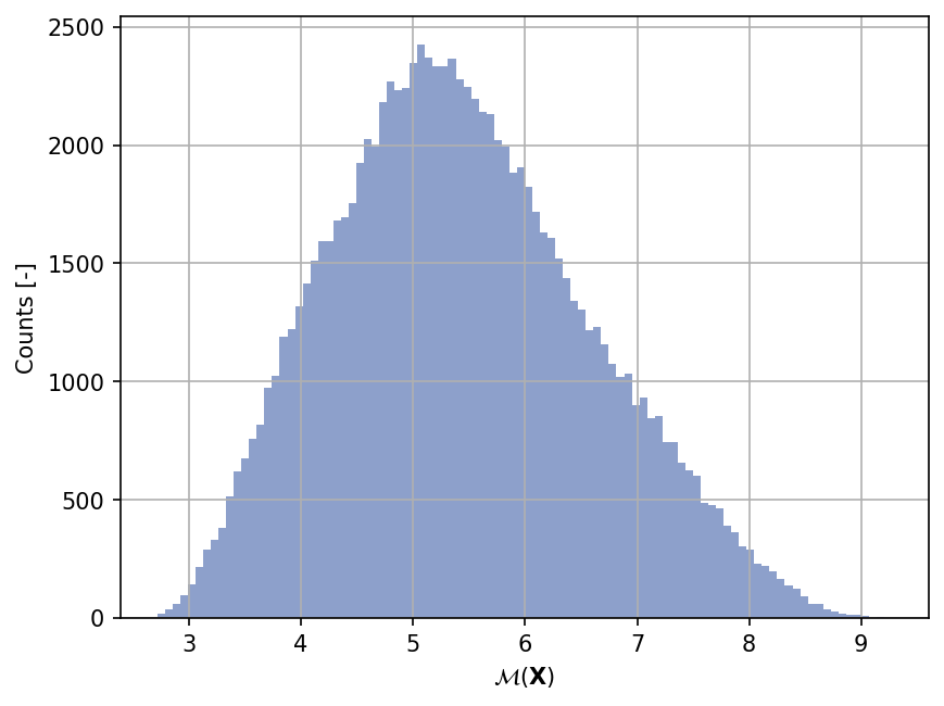
Sample histogram

Shown below is the histogram of the output based on \(100'000\) random points:

Show code cell source Hide code cell source

np.random.seed(42)
xx_test = my_testfun.prob_input.get_sample(100000)
yy_test = my_testfun(xx_test)

plt.hist(yy_test, bins="auto", color="#8da0cb");
plt.grid();
plt.ylabel("Counts [-]");
plt.xlabel("$\mathcal{M}(\mathbf{X})$");
plt.gcf().set_dpi(150);

Moments estimation

Shown below is the convergence of a direct Monte-Carlo estimation of the output mean and variance with increasing sample sizes.

Show code cell source Hide code cell source

# --- Compute the mean and variance estimate
np.random.seed(42)
sample_sizes = np.array([1e1, 1e2, 1e3, 1e4, 1e5, 1e6, 1e7], dtype=int)
mean_estimates = np.empty(len(sample_sizes))
var_estimates = np.empty(len(sample_sizes))

for i, sample_size in enumerate(sample_sizes):
    xx_test = my_testfun.prob_input.get_sample(sample_size)
    yy_test = my_testfun(xx_test)
    mean_estimates[i] = np.mean(yy_test)
    var_estimates[i] = np.var(yy_test)

# --- Compute the error associated with the estimates
mean_estimates_errors = np.sqrt(var_estimates) / np.sqrt(np.array(sample_sizes))
var_estimates_errors = var_estimates * np.sqrt(2 / (np.array(sample_sizes) - 1))

# --- Do the plot
fig, ax_1 = plt.subplots(figsize=(6,4))

ax_1.errorbar(
    sample_sizes,
    mean_estimates,
    yerr=mean_estimates_errors,
    marker="o",
    color="#66c2a5",
    label="Mean",
)
ax_1.set_xlabel("Sample size")
ax_1.set_ylabel("Output mean estimate")
ax_1.set_xscale("log");
ax_2 = ax_1.twinx()
ax_2.errorbar(
    sample_sizes + 1,
    var_estimates,
    yerr=var_estimates_errors,
    marker="o",
    color="#fc8d62",
    label="Variance",
)
ax_2.set_ylabel("Output variance estimate")

# Add the two plots together to have a common legend
ln_1, labels_1 = ax_1.get_legend_handles_labels()
ln_2, labels_2 = ax_2.get_legend_handles_labels()
ax_2.legend(ln_1 + ln_2, labels_1 + labels_2, loc=0)

plt.grid()
fig.set_dpi(150)

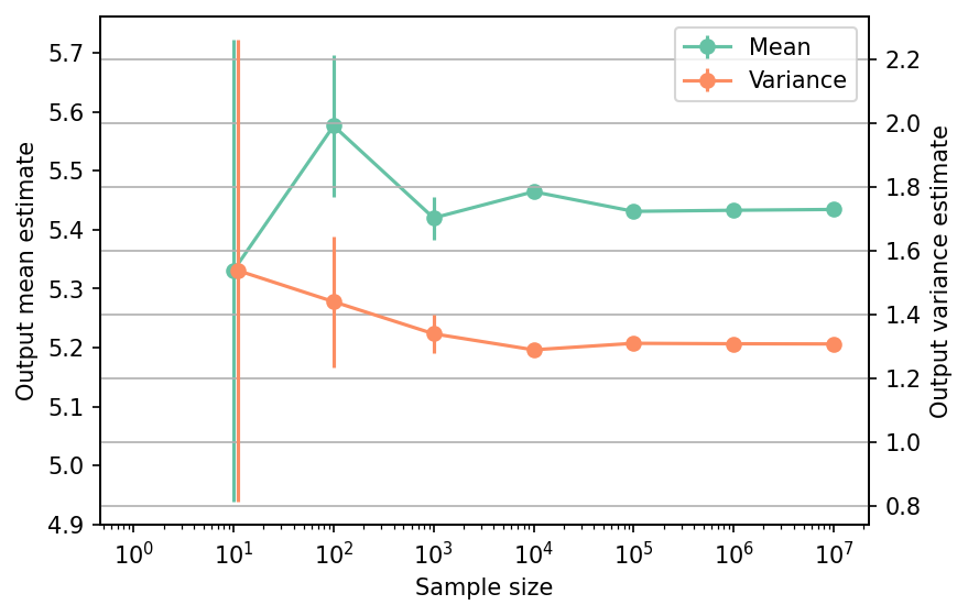
The tabulated results for is shown below.

Show code cell source Hide code cell source

from tabulate import tabulate

# --- Compile data row-wise
outputs = []
for (
    sample_size,
    mean_estimate,
    mean_estimate_error,
    var_estimate,
    var_estimate_error,
) in zip(
    sample_sizes,
    mean_estimates,
    mean_estimates_errors,
    var_estimates,
    var_estimates_errors,
):
    outputs += [
        [
            sample_size,
            mean_estimate,
            mean_estimate_error,
            var_estimate,
            var_estimate_error,
            "Monte-Carlo",
        ],
    ]

header_names = [
    "Sample size",
    "Mean",
    "Mean error",
    "Variance",
    "Variance error",
    "Remark",
]

tabulate(
    outputs,
    headers=header_names,
    floatfmt=(".1e", ".4f", ".4e", ".4f", ".4e", "s"),
    tablefmt="html",
    stralign="center",
    numalign="center",
)

Sample size	Mean	Mean error	Variance	Variance error	Remark
1.0e+01	5.3309	3.9209e-01	1.5373	7.2470e-01	Monte-Carlo
1.0e+02	5.5764	1.1996e-01	1.4390	2.0453e-01	Monte-Carlo
1.0e+03	5.4201	3.6588e-02	1.3387	5.9898e-02	Monte-Carlo
1.0e+04	5.4646	1.1351e-02	1.2884	1.8221e-02	Monte-Carlo
1.0e+05	5.4313	3.6178e-03	1.3088	5.8532e-03	Monte-Carlo
1.0e+06	5.4331	1.1434e-03	1.3074	1.8489e-03	Monte-Carlo
1.0e+07	5.4345	3.6150e-04	1.3068	5.8442e-04	Monte-Carlo

References

[Moo10] (1,2,3,4,5)

Hyejung Moon. Design and analysis of computer experiments for screening input variables. PhD thesis, Ohio State University, Ohio, 2010. URL: http://rave.ohiolink.edu/etdc/view?acc_num=osu1275422248.

[BAS07] (1,2,3)

Einat Neumann Ben-Ari and David M. Steinberg. Modeling data from computer experiments: an empirical comparison of kriging with MARS and projection pursuit regression. Quality Engineering, 19(4):327–338, 2007. doi:10.1080/08982110701580930.