Moon (2010) Three-Dimensional Function#
import numpy as np
import matplotlib.pyplot as plt
import uqtestfuns as uqtf
The three-dimensional function from [Moo10] (or Moon3D for short)
is a scalar-valued test function used in [Moo10] to illustrate
the analytical derivation of Sobol’ sensitivity indices.
Test function instance#
To create an instance of the test function:
my_testfun = uqtf.Moon3D()
Check if it has been correctly instantiated:
print(my_testfun)
Function ID      : Moon3D
Input Dimension  : 3 (fixed)
Output Dimension : 1
Parameterized    : False
Description      : Three-dimensional function from Moon (2010)
Applications     : sensitivity
Description#
The function Moon3D is a three-dimensional function given by the following
formula[1]:
where \(\boldsymbol{x} = \{ x_1, x_2, x_3 \}\) is the three-dimensional vector of input variables further defined below.
Probabilistic input#
Based on [Moo10], the probabilistic input model for the function consists of three independent uniform random variables with the ranges shown in the table below.
Show code cell source
print(my_testfun.prob_input)
Function ID     : Moon3D
Input ID        : Moon2010
Input Dimension : 3
Description     : Probabilistic input model for the 3D test function from
                  Moon (2010)
Marginals       :

 No.    Name    Distribution    Parameters    Description
-----  ------  --------------  ------------  -------------
  1      X1       uniform         [0 1]            -
  2      X2       uniform         [0 1]            -
  3      X3       uniform         [0 1]            -

Copulas         : Independence
Reference results#
This section provides several reference results of typical UQ analyses involving the test function.
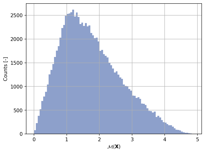
Sample histogram#
Shown below is the histogram of the output based on \(100'000\) random points:
Show code cell source
np.random.seed(42)
xx_test = my_testfun.prob_input.get_sample(100000)
yy_test = my_testfun(xx_test)

plt.hist(yy_test, bins="auto", color="#8da0cb");
plt.grid();
plt.ylabel("Counts [-]");
plt.xlabel("$\mathcal{M}(\mathbf{X})$");
plt.gcf().set_dpi(150);
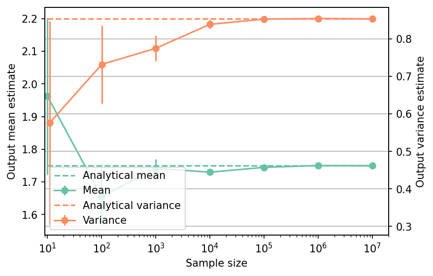
Moment estimations#
The mean and variance of the test function can be computed analytically,
and the results are:
\(\mathbb{E}[Y] = \frac{7}{4}\)
\(\mathbb{V}[Y] = \frac{41}{48}\)
Shown below is the convergence of a direct Monte-Carlo estimation of the output mean and variance with increasing sample sizes compared with the analytical values.
Show code cell source
# --- Compute the mean and variance estimate
np.random.seed(42)
sample_sizes = np.array([1e1, 1e2, 1e3, 1e4, 1e5, 1e6, 1e7], dtype=int)
mean_estimates = np.empty(len(sample_sizes))
var_estimates = np.empty(len(sample_sizes))

for i, sample_size in enumerate(sample_sizes):
    xx_test = my_testfun.prob_input.get_sample(sample_size)
    yy_test = my_testfun(xx_test)
    mean_estimates[i] = np.mean(yy_test)
    var_estimates[i] = np.var(yy_test)

# --- Compute the error associated with the estimates
mean_estimates_errors = np.sqrt(var_estimates) / np.sqrt(np.array(sample_sizes))
var_estimates_errors = var_estimates * np.sqrt(2 / (np.array(sample_sizes) - 1))

fig, ax_1 = plt.subplots(figsize=(6,4))

# --- Mean plot
ax_1.errorbar(
    sample_sizes,
    mean_estimates,
    yerr=mean_estimates_errors,
    marker="o",
    color="#66c2a5",
    label="Mean"
)
# Plot the analytical mean
mean_analytical = 7/4
ax_1.plot(
    sample_sizes,
    np.repeat(mean_analytical, len(sample_sizes)),
    linestyle="--",
    color="#66c2a5",
    label="Analytical mean",
)
ax_1.set_xlim([9, 2e7])
ax_1.set_xlabel("Sample size")
ax_1.set_ylabel("Output mean estimate")
ax_1.set_xscale("log");
ax_2 = ax_1.twinx()

# --- Variance plot
ax_2.errorbar(
    sample_sizes+1,
    var_estimates,
    yerr=var_estimates_errors,
    marker="o",
    color="#fc8d62",
    label="Variance",
)
# Plot the analytical variance
var_analytical = 41/48
ax_2.plot(
    sample_sizes,
    np.repeat(var_analytical, len(sample_sizes)),
    linestyle="--",
    color="#fc8d62",
    label="Analytical variance",
)
ax_2.set_ylabel("Output variance estimate")

# Add the two plots together to have a common legend
ln_1, labels_1 = ax_1.get_legend_handles_labels()
ln_2, labels_2 = ax_2.get_legend_handles_labels()
ax_2.legend(ln_1 + ln_2, labels_1 + labels_2, loc=0)

plt.grid()
fig.set_dpi(150)
The tabulated results for each sample size is shown below.
Show code cell source
from tabulate import tabulate

# --- Compile data row-wise
outputs = [
    [
        np.nan,
        mean_analytical,
        0.0,
        var_analytical,
        0.0,
        "Analytical",
    ]
]

for (
    sample_size,
    mean_estimate,
    mean_estimate_error,
    var_estimate,
    var_estimate_error,
) in zip(
    sample_sizes,
    mean_estimates,
    mean_estimates_errors,
    var_estimates,
    var_estimates_errors,
):
    outputs += [
        [
            sample_size,
            mean_estimate,
            mean_estimate_error,
            var_estimate,
            var_estimate_error,
            "Monte-Carlo",
        ],
    ]

header_names = [
    "Sample size",
    "Mean",
    "Mean error",
    "Variance",
    "Variance error",
    "Remark",
]

tabulate(
    outputs,
    headers=header_names,
    floatfmt=(".1e", ".4e", ".4e", ".4e", ".4e", "s"),
    tablefmt="html",
    stralign="center",
    numalign="center",
)
| Sample size | Mean | Mean error | Variance | Variance error | Remark |
|---|---|---|---|---|---|
| nan | 1.7500e+00 | 0.0000e+00 | 8.5417e-01 | 0.0000e+00 | Analytical |
| 1.0e+01 | 1.9629e+00 | 2.4008e-01 | 5.7639e-01 | 2.7172e-01 | Monte-Carlo |
| 1.0e+02 | 1.6547e+00 | 8.5583e-02 | 7.3244e-01 | 1.0410e-01 | Monte-Carlo |
| 1.0e+03 | 1.7418e+00 | 2.7846e-02 | 7.7542e-01 | 3.4695e-02 | Monte-Carlo |
| 1.0e+04 | 1.7298e+00 | 9.1613e-03 | 8.3930e-01 | 1.1870e-02 | Monte-Carlo |
| 1.0e+05 | 1.7447e+00 | 2.9212e-03 | 8.5334e-01 | 3.8163e-03 | Monte-Carlo |
| 1.0e+06 | 1.7502e+00 | 9.2465e-04 | 8.5497e-01 | 1.2091e-03 | Monte-Carlo |
| 1.0e+07 | 1.7500e+00 | 2.9224e-04 | 8.5405e-01 | 3.8194e-04 | Monte-Carlo |
Sensitivity indices#
The main-effect and total-effect Sobol’ indices of the test function can be
derived analytically.
Input |
Main-effect (\(S_i\)) |
Total-effect (\(ST_i\)) |
|---|---|---|
\(x_1\) |
\(\frac{25}{41}\) |
\(\frac{28}{41}\) |
\(x_2\) |
\(\frac{4}{41}\) |
\(\frac{4}{41}\) |
\(x_3\) |
\(\frac{9}{41}\) |
\(\frac{12}{41}\) |
References#
Hyejung Moon. Design and analysis of computer experiments for screening input variables. PhD thesis, Ohio State University, Ohio, 2010. URL: http://rave.ohiolink.edu/etdc/view?acc_num=osu1275422248.