Eight-Dimensional Function from Dette and Pepelyshev (2010)#
import numpy as np
import matplotlib.pyplot as plt
import uqtestfuns as uqtf
The function is a three-dimensional, scalar-valued function. The function include the curved term from the curved function and an additional logarithm term. It is highly curved with respect to some input variables and less so with respect to the others.
The function appeared in [DP10] as a test function for comparing different experimental designs in the construction of metamodels.
Test function instance#
To create a default instance of the test function:
my_testfun = uqtf.Dette8D()
Check if it has been correctly instantiated:
print(my_testfun)
Function ID      : Dette8D
Input Dimension  : 8 (fixed)
Output Dimension : 1
Parameterized    : False
Description      : 8D function from Dette and Pepelyshev (2010)
Applications     : metamodeling
Description#
The test function is defined as[1]:
where \(\boldsymbol{x} = \left( x_1, x_2, x_3 \right)\) is the three-dimensional vector of input variables further defined below. Notice that the term before the logarithm term is the terms from the curved function.
Probabilistic input#
The probabilistic input model for the test function is shown below.
Show code cell source
print(my_testfun.prob_input)
Function ID     : DetteCurved
Input ID        : Dette2010
Input Dimension : 8
Description     : Input specification for the 8D test function from Dette
                  and Pepelyshev (2010)
Marginals       :

 No.    Name    Distribution    Parameters    Description
-----  ------  --------------  ------------  -------------
  1     x_1       uniform         [0 1]            -
  2     x_2       uniform         [0 1]            -
  3     x_3       uniform         [0 1]            -
  4     x_4       uniform         [0 1]            -
  5     x_5       uniform         [0 1]            -
  6     x_6       uniform         [0 1]            -
  7     x_7       uniform         [0 1]            -
  8     x_8       uniform         [0 1]            -

Copulas         : Independence
Reference results#
This section provides several reference results of typical UQ analyses involving the test function.
Sample histogram#
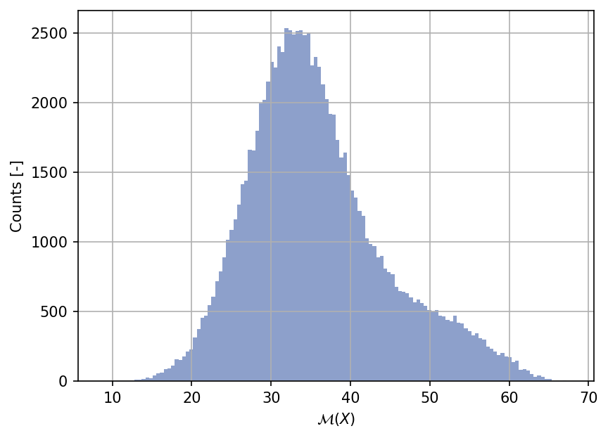
Shown below is the histogram of the output based on \(100'000\) random points:
Show code cell source
my_testfun.prob_input.reset_rng(42)
xx_test = my_testfun.prob_input.get_sample(100000)
yy_test = my_testfun(xx_test)

plt.hist(yy_test, bins="auto", color="#8da0cb");
plt.grid();
plt.ylabel("Counts [-]");
plt.xlabel("$\mathcal{M}(X)$");
plt.gcf().tight_layout(pad=3.0)
plt.gcf().set_dpi(150);
References#
Holger Dette and Andrey Pepelyshev. Generalized latin hypercube design for computer experiments. Technometrics, 52(4):421–429, 2010. doi:10.1198/tech.2010.09157.