Tutorial: Create a Custom Test Function

Tutorial: Create a Custom Test Function#

You may add an uncertainty quantification (UQ) test functions to UQTestFuns such that they share the same interface like the built-in ones. There are two ways to add a new test function to UQTestFuns:

Interactively within a given Python session; if not saved, the test function will be gone after a new session.
Updating the package by implementing the function in a new module within the UQTestFuns package; the test function will available after importing the package.

In this tutorial, you’ll learn how to add a test function interactively. If you want to add a new test function as a Python module, please refer to the relevant section in the Developer’s Guide.

import numpy as np
import uqtestfuns as uqtf

Uncertainty quantification test functions revisited#

In essence, an uncertainty quantification (UQ) test function contains the following components:

an evaluation function that takes inputs and produces outputs; we can think of such functions as a blackbox
a probabilistic input model that specifies the input to the blackbox function as a joint random variable; the results of a UQ analysis depend on this specification
(optionally) a set of parameters that completes the test function specification; these parameters once set are kept during the function evaluation (for example, flag, numerical tolerance, and time-step size).

When defining a new generic UQ test function, it’s a good idea to think about the candidate test function in those three terms and be ready with their specifications.

Branin function#

Suppose we want to add the two-dimensional Branin (or Branin-Hoo) function as a test function [DS78]. The function is defined analytically as follows:

\[ \mathcal{M}(x_1, x_2) = a \left( x_2 - b x_1^2 + c x_1 - r \right)^2 + s \left(1 - t \right) \cos{(x_1}) + s \]

where \(x_1\) and \(x_2\) are the input variables and \(\{ a, b, c, r, s, t \}\) are the parameters.

The input variables are defined in the table below.

No.	Name	Distribution	Parameters
1	\(x_1\)	uniform	\([-5, 10]\)
2	\(x_2\)	uniform	\([0, 15]\)

The typical values for the parameters are shown in the table below.

No.	Parameter	Value
1	\(a\)	\(1.0\)
2	\(b\)	\(\frac{5.1}{(2 \pi)^2}\)
3	\(c\)	\(\frac{5}{\pi}\)
4	\(r\)	\(6\)
5	\(s\)	\(10\)
6	\(t\)	\(\frac{1}{8 \pi}\)

Evaluation function#

The first component of a test function is the evaluation function itself. UQTestFuns requires for such a function to have at least the input array as its first parameter. When applicable, the parameters must appear after the input array. It’s your choice whether to lump the parameters together or split them as exemplified below. The Branin evaluation function can be defined as a Python function as follows:

def evaluate_branin(xx: np.ndarray, a: float, b: float, c: float, r: float, s: float, t: float):
    """Evaluate the Branin function on a set of input values.
    
    Parameters
    ----------
    xx : np.ndarray
        2-Dimensional input values given by an N-by-2 array where
        N is the number of input values.
    a : float
        Parameter 'a' of the Branin function.
    b : float
        Parameter 'b' of the Branin function.
    c : float
        Parameter 'c' of the Branin function.
    r : float
        Parameter 'r' of the Branin function.
    s : float
        Parameter 's' of the Branin function.
    t : float
        Parameter 't' of the Branin function.
    
    Returns
    -------
    np.ndarray
        The output of the Branin function evaluated on the input values.
        The output is a 1-dimensional array of length N.    
    """
    yy = (
        a * (xx[:, 1] - b * xx[:, 0]**2 + c * xx[:, 0] - r)**2
        + s * (1 - t) * np.cos(xx[:, 0]) 
        + s
    )
    
    return yy

Input and parameters#

The second a test function is the (probabilistic) input specification. The input specification of the Branin function consists of two independent uniform random variables with different bounds. In UQTestFuns, a probabilistic input model is represented by the the ProbInput class and an instance of it can be defined as follows:

# Define a list of marginals
marginals = [
    uqtf.Marginal(distribution="uniform", parameters=[-5, 10], name="x1"),
    uqtf.Marginal(distribution="uniform", parameters=[0, 15], name="x2"),
]
# Create a probabilistic input
my_input = uqtf.ProbInput(marginals=marginals, function_id="Branin", input_id="custom")

To verify if the instance has been created successfully, print it out to the terminal:

print(my_input)

Function ID     : Branin
Input ID        : custom
Input Dimension : 2
Description     : -
Marginals       :

 No.    Name    Distribution    Parameters    Description
-----  ------  --------------  ------------  -------------
  1      x1       uniform        [-5 10]           -
  2      x2       uniform        [ 0 15]           -

Copulas         : Independence

Parameters#

The third and final component of a test function is the parameter set. A test function may or may not have a parameter set; in the case of the Branin function, the set contains six parameters \(\{ a, b, c, r, s, t \}\).

A parameter set in UQTestFuns is represented by the FunParams class. As defined above, the test function requires six separate parameters. An instance of FunParams can be created as follows:

my_params = uqtf.FunParams(
    function_id="Branin",
    parameter_id="custom",
    description="Parameter set for the Branin function",
)

Each of the parameters can then be added to the set as follows:

my_params.add(keyword="a", value=1.0, type=float)
my_params.add(keyword="b", value=5.1 / (2 * np.pi)**2, type=float)
my_params.add(keyword="c", value=5 / np.pi, type=float)
my_params.add(keyword="r", value=6.0, type=float)
my_params.add(keyword="s", value=10.0, type=float)
my_params.add(keyword="t", value=1 / (8 * np.pi), type=float)

Notice that the values to the keyword parameter are consistent with the names that appear in the function definition The value of the parameters can practically be of any Python data type. They only depend on how they are going to be consumed by the specified evaluatuon function.

Note

The type parameter is optional; when specified the set value must be consistent.

To verify if the instance has been created successfully, print it out to the terminal:

print(my_params)

Function ID  : Branin
Parameter ID : custom
Description  : Parameter set for the Branin function

 No.    Keyword      Value      Type    Description
-----  ---------  -----------  ------  -------------
  1        a      1.00000e+00  float         -
  2        b      1.29185e-01  float         -
  3        c      1.59155e+00  float         -
  4        r      6.00000e+00  float         -
  5        s      1.00000e+01  float         -
  6        t      3.97887e-02  float         -

Creating a test function#

The evaluation function, probabilistic input, and parameters are combined to make a test function via the UQTestFun class. An instance of the class for the Branin function is written as follows:

my_testfun = uqtf.UQTestFun(
  evaluate=evaluate_branin,
  prob_input=my_input,
  parameters=my_params,
  function_id="Branin",
)

Print the resulting instance to the terminal to verify:

print(my_testfun)

Function ID      : Branin
Input Dimension  : 2
Output Dimension : 1
Parameterized    : True

Congratulations! You’ve successfully created a test function instance of the Branin function inside a Python session. This instance can be evaluated as a usual function. Below are the surface and contour plots of the test function; both require function evaluation on the grid.

../_images/5ad5b63db2233af1f778e980a53cbc4493d97b2b1d98284748632ec16e123a20.png

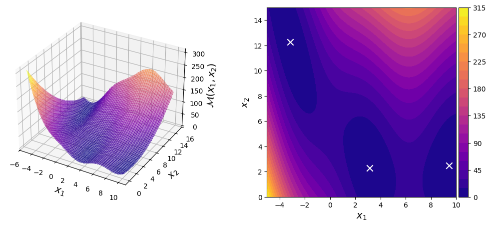
The Branin function is a test function typically used for testing optimization algorithms. Shown in the contour plot above are the locations of the three global optima of the function.

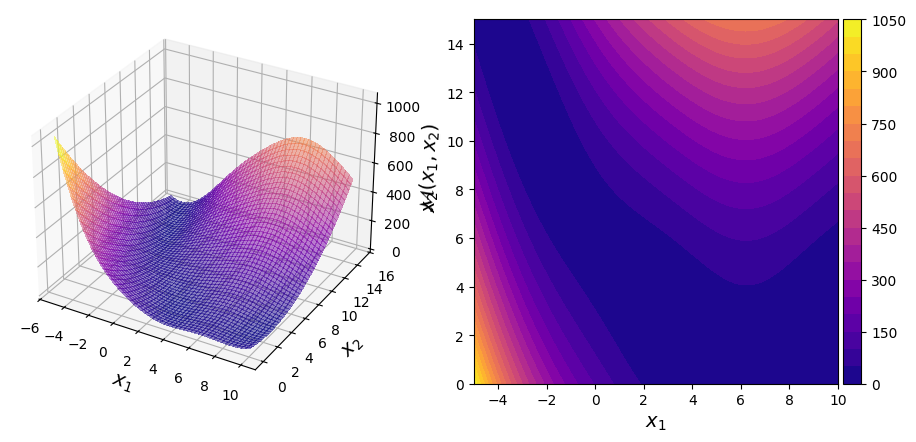
You can change the value of the parameters on the fly by accessing the parameter by its keyword. For example:

my_testfun.parameters["a"] = 3.5
my_testfun.parameters["t"] = 1 / (4 * np.pi)

which will alter the landscape.

../_images/1e7926ad7162d2751db539506f5e2946c4ade726f1dfafc385579616c1f53dcc.png

Concluding remarks#

The test function created above only persists in the current Python session. To use the same Branin test function in another session, you can either repeat the same procedure (for example, via a script) or save it into an object in the disk and load it in the new session.

Alternatively, you can extend UQTestFuns directly by specifying the test function inside its own module. This way, once UQTestFuns is loaded you can construct the test function like any other built-in test function. For example, if you somehow name the test function Branin then:

my_testfun = uqtf.Branin()

will construct an instance of the Branin function using the default input and parameter values.

You can find a guide on how to do this in more detail in the relevant section of the Developer’s Guide.

[1]

L. C. W. Dixon and G. P. Szegö. Towards global optimization 2, chapter The global optimization problem: an introduction, pages 1–15. North-Holland, Amsterdam, 1978.