Bratley et al. (1992) B function#
import numpy as np
import matplotlib.pyplot as plt
import uqtestfuns as uqtf
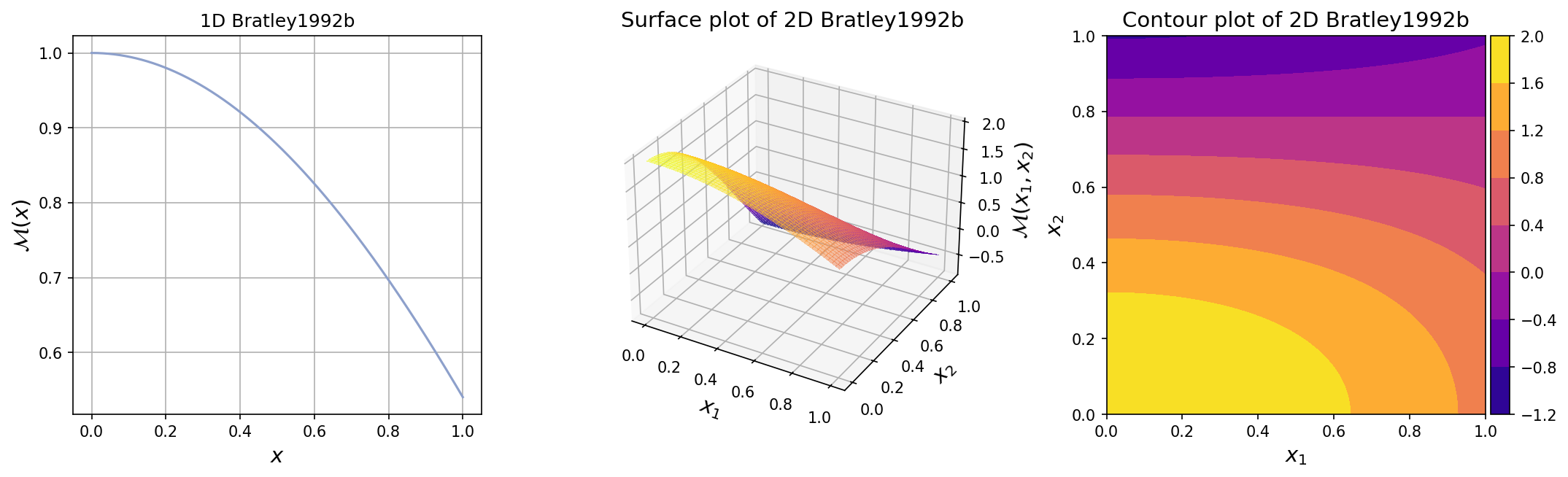
The Bratley et al. (1992) B function (or Bratley1992b function for short),
is an \(M\)-dimensional scalar-valued function.
The function was introduced in [BFN92] as a test function
for multi-dimensional numerical integration using low discrepancy sequences.
Note
There are four other test functions used in Bratley et al. [BFN92]:
Bratley et al. (1992) A: A product of an absolute function
Bratley et al. (1992) B: A product of a trigonometric function (this function)
Bratley et al. (1992) C: A product of the Chebyshev polynomial of the first kind
Bratley et al. (1992) D: A sum of product
The plots for one-dimensional and two-dimensional Bratley1992b functions
are shown below.
Test function instance#
To create a default instance of the test function:
my_testfun = uqtf.Bratley1992b()
Check if it has been correctly instantiated:
print(my_testfun)
Function ID      : Bratley1992b
Input Dimension  : 2 (variable)
Output Dimension : 1
Parameterized    : False
Description      : Integration test function #2 from Bratley et al. (1992)
Applications     : integration, sensitivity
By default, the input dimension is set to \(2\)[1].
To create an instance with another value of input dimension,
pass an integer to the parameter input_dimension (keyword only).
For example, to create an instance of 10-dimensional Bratley1992b function,
type:
my_testfun = uqtf.Bratley1992b(input_dimension=10)
Description#
The Bratley1992b function is defined as follows[2]:
where \(\boldsymbol{x} = \{ x_1, \ldots, x_M \}\) is the \(M\)-dimensional vector of input variables further defined below.
Probabilistic input#
Based on [BFN92], the test function is integrated over the hypercube domain of \([0, 1]^M\). Such an input specification can be modeled using an \(M\) independent uniform random variables as shown in the table below.
No. |
Name |
Distribution |
Parameters |
Description |
|---|---|---|---|---|
1 |
\(x_1\) |
uniform |
[0.0 1.0] |
N/A |
\(\vdots\) |
\(\vdots\) |
\(\vdots\) |
\(\vdots\) |
\(\vdots\) |
M |
\(x_M\) |
uniform |
[0.0 1.0] |
N/A |
Reference results#
This section provides several reference results of typical UQ analyses involving the test function.
Definite integration#
The integral value of the function over the domain of \([0.0, 1.0]^M\) is analytical:
The table below shows the numerical values of the integral for several selected dimensions.
Dimension |
\(I[\mathcal{M}]\) |
|---|---|
1 |
\(8.4147098 \times 10^{-1}\) |
2 |
\(7.6514740 \times 10^{-1}\) |
3 |
\(1.0797761 \times 10^{-1}\) |
4 |
\(-8.1717723 \times 10^{-2}\) |
5 |
\(7.8361108 \times 10^{-2}\) |
6 |
\(-2.1895308 \times 10^{-2}\) |
7 |
\(-1.4384924 \times 10^{-2}\) |
8 |
\(-1.4231843 \times 10^{-2}\) |
9 |
\(-5.8652056 \times 10^{-3}\) |
10 |
\(3.1907957 \times 10^{-3}\) |
The absolute value of the integral is monotonically decreasing function of the number of dimensions. Asymptotically, it is zero. In the original paper of Bratley [BFN92], the integration was carried out for the function in dimension eight.
Moments#
The moments of the test function are analytically known and the first two moments are given below.
Expected value#
Due to the domain being a hypercube, the above integral value over the domain is the same as the expected value:
Variance#
The analytical value for the variance is given as follows:
The table below shows the numerical values of the variance for several selected dimensions.
Dimension |
\(I[\mathcal{M}]\) |
|---|---|
1 |
\(1.9250938 \times 10^{-2}\) |
2 |
\(5.9397772 \times 10^{-1}\) |
3 |
\(5.0486051 \times 10^{0}\) |
4 |
\(4.5481851 \times 10^{1}\) |
5 |
\(5.3766707 \times 10^{2}\) |
6 |
\(9.245366 \times 10^{3}\) |
7 |
\(2.4253890 \times 10^{5}\) |
8 |
\(7.6215893 \times 10^{6}\) |
9 |
\(2.9579601 \times 10^{8}\) |
10 |
\(1.5464914 \times 10^{10}\) |
The variance grows as the number of dimensions and becomes unbounded for a very large dimension.