Single-Diode Solar Cell Model#
import numpy as np
import matplotlib.pyplot as plt
import uqtestfuns as uqtf
The test function is a five-dimensional, scalar-valued function that models the maximum power of a single-diode solar cell. The function was used in [CZC15] to demonstrate the active subspace method for input dimension reduction and sensitivity analysis.
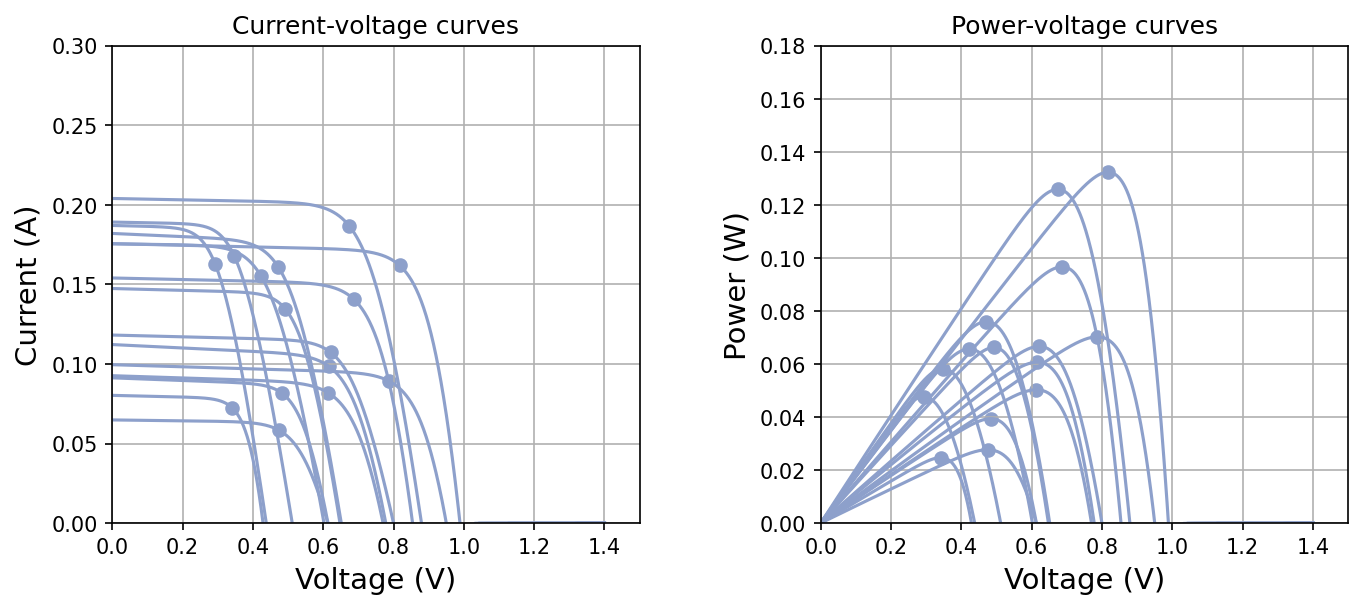
For a given voltage, the corresponding current is defined implicitly. The plot below (left) displays 15 current-voltage curves from 15 different input variable values. The dots on the curves indicate the current and voltage values that yield the maximum cell power; the power curves are shown in the right plot.
Test function instance#
To create a default instance of the test function:
my_testfun = uqtf.SolarCell()
Check if it has been correctly instantiated:
print(my_testfun)
Function ID      : SolarCell
Input Dimension  : 5 (fixed)
Output Dimension : 1
Parameterized    : True
Description      : Single-diode solar-cell model from Constantine et al. (2015)
Applications     : metamodeling, sensitivity
Description#
The model predicts the maximum power of a single-diode solar cell defined in the following formula:
where the current (\(I\)) is defined implicitly as a function of the voltage (\(V\)), input variables \(\boldsymbol{x}\) and parameters \(\boldsymbol{p}\). The implicit relationshow is described by the following equation:
where \(I_L\), the photocurrent, is defined by the auxiliary equation:
Here, \(\boldsymbol{x} = \left( I_{SC}, I_S, n, R_S, R_P \right)\) represents the five-dimensional the vector of input variables probabilistically defined below. The vector \(\boldsymbol{p} = \left( n_s, V_{\text{th}} \right)\) contains fixed parameters, which are also further detailed below.
Probabilistic input#
The probabilistic input model for the test function is shown below.
Show code cell source
print(my_testfun.prob_input)
Function ID     : SolarCell
Input ID        : Constantine2015
Input Dimension : 5
Description     : Probabilistic input model for the single-diode solar cell
                  model from Constantine et al. (2015)
Marginals       :

 No.    Name    Distribution           Parameters                          Description
-----  ------  --------------  ---------------------------  ------------------------------------------
  1     Isc       uniform           [0.05989 0.23958]               Short-circuit current [A]
  2    log_Is     uniform      [-24.53997866 -15.32963829]  (log) Diode reverse saturation current [A]
  3      n        uniform                [1. 2.]                       Ideality factor [-]
  4      Rs       uniform           [0.16625 0.665  ]                Series resistance [Ohm]
  5      Rp       uniform            [ 93.75 375.  ]            Parallel (shunt) resistance [Ohm]

Copulas         : Independence
Parameters#
The default values of the parameters are shown below.
Show code cell source
print(my_testfun.parameters)
Function ID  : SolarCell
Parameter ID : Constantine2015
Description  : Parameter set for the single-diode solar cell model from
               Constantine et al. (2015)

 No.    Keyword      Value      Type              Description
-----  ---------  -----------  ------  ----------------------------------
  1       n_s     1.00000e+00   int    # of cells connected in series [-]
  2      v_th     2.58500e-02  float     Thermal voltage at 25degC [V]
Reference results#
This section provides several reference results of typical UQ analyses involving the test function.
Sample histogram#
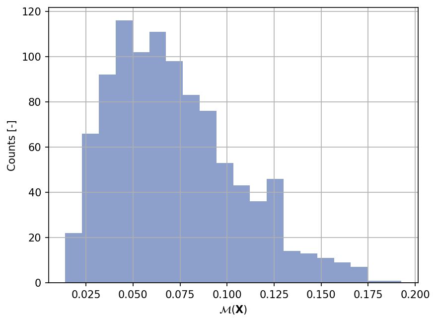
Shown below is the histogram of the output based on \(1000\) random points:
Show code cell source
xx_test = my_testfun.prob_input.get_sample(1000)
yy_test = my_testfun(xx_test)

plt.hist(yy_test, bins="auto", color="#8da0cb");
plt.grid();
plt.ylabel("Counts [-]");
plt.xlabel("$\mathcal{M}(\mathbf{X})$");
plt.gcf().set_dpi(150);
Notes on numerical algorithms#
The maximum power of the solar cell model is computed numerically using the following methods:
root()from SciPy, with its default method and parameter values, to solve the implicit current as a function of voltage.minimize()from SciPy, with its default method (i.e.,BFGS) and parameter values, to find the maximum power by optimizing over the voltage (the current is is computed on-the-fly during the iteration).
The default parameter values for these methods can be overridden by providing a dictionary with new parameter values. For example:
To override the tolerance value for root():
fun.parameters.add("root", {"tol": 1e-12}) # 'root' as the parameter keyword
To override the tolerance value for minimize():
fun.parameters.add("minimize", {"tol": 1e-12}) # 'minimize' as the parameter keyword
Note
In this example, tol is acceptable keyword-named argument for both root()
and minimize(); indeed, the key-value pairs specified for the parameters
root and minimize must be recognized by the respective methods.
References#
Paul G. Constantine, Brian Zaharatos, and Mark Campanelli. Discovering an active subspace in a single‐diode solar cell model. Statistical Analysis and Data Mining: The ASA Data Science Journal, 8(5–6):264–273, ] 2015. doi:10.1002/sam.11281.