Bratley et al. (1992) C function

Bratley et al. (1992) C function#

import numpy as np
import matplotlib.pyplot as plt
import uqtestfuns as uqtf

The Bratley et al. (1992) C function (or Bratley1992c function for short), is an \(M\)-dimensional scalar-valued function. The function was introduced in [BFN92] as a test function for multi-dimensional numerical integration using low discrepancy sequences.

Note

There are four other test functions used in Bratley et al. [BFN92]:

Bratley et al. (1992) A: A product of an absolute function
Bratley et al. (1992) B: A product of a trigonometric function
Bratley et al. (1992) C: A product of the Chebyshev polynomial of the first kind (this function)
Bratley et al. (1992) D: A sum of product

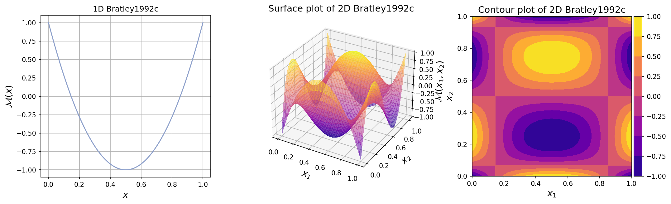
The plots for one-dimensional and two-dimensional Bratley1992c functions are shown below.

../_images/70e3987d7fb59d8336bcff9e167087a372d6388498729a5a0ea738d70a871056.png

Test function instance#

To create a default instance of the test function:

my_testfun = uqtf.Bratley1992c()

Check if it has been correctly instantiated:

print(my_testfun)

Function ID      : Bratley1992c
Input Dimension  : 2 (variable)
Output Dimension : 1
Parameterized    : False
Description      : Integration test function #3 from Bratley et al. (1992)
Applications     : integration, sensitivity

By default, the input dimension is set to \(2\)[1]. To create an instance with another value of input dimension, pass an integer to the parameter input_dimension (keyword only). For example, to create an instance of 10-dimensional Bratley1992c function, type:

my_testfun = uqtf.Bratley1992c(input_dimension=10)

Description#

The Bratley1992c function is defined as follows[2]:

\[ \mathcal{M}(\boldsymbol{x}) = \prod_{m = 1}^M T_{n_m} (2 x_m - 1) \]

where \(T_{n_m}\) is the Chebyshev polynomial (of the first kind) of degree \(n_m\), \(n_m = m \bmod 4 + 1\), and \(\boldsymbol{x} = \{ x_1, \ldots, x_M \}\) is the \(M\)-dimensional vector of input variables further defined below.

Probabilistic input#

Based on [BFN92], the test function is integrated over the hypercube domain of \([0, 1]^M\). Such an input specification can be modeled using an \(M\) independent uniform random variables as shown in the table below.

No.	Name	Distribution	Parameters	Description
1	\(x_1\)	uniform	[0.0 1.0]	N/A
\(\vdots\)	\(\vdots\)	\(\vdots\)	\(\vdots\)	\(\vdots\)
M	\(x_M\)	uniform	[0.0 1.0]	N/A

Reference results#

This section provides several reference results of typical UQ analyses involving the test function.

Definite integration#

The integral value of the function over the domain of \([0.0, 1.0]^M\) is analytical:

\[\begin{split} I[\mathcal{M}] (M) \equiv \int_{[0, 1]^M} \mathcal{M}(\boldsymbol{x}) \; d\boldsymbol{x} = \begin{cases} -\frac{1}{3}, & M = 1 \\ 0, & M \neq 1 \end{cases}. \end{split}\]

Due to the domain being a hypercube, the above integral value over the domain is the same as the expected value.

References#

[BFN92] (1,2,3,4)

Paul Bratley, Bennett L. Fox, and Harald Niederreiter. Implementation and tests of low-discrepancy sequences. ACM Transactions on Modeling and Computer Simulation, 2(3):195–213, 1992. doi:10.1145/146382.146385.