Bratley et al. (1992) D function#
import numpy as np
import matplotlib.pyplot as plt
import uqtestfuns as uqtf
The Bratley et al. (1992) D function (or Bratley1992d function for short),
is an \(M\)-dimensional scalar-valued function.
The function was introduced in [BFN92] as a test function
for multi-dimensional numerical integration using low discrepancy sequences.
It was used in [KRFPS09] and [SAA+10] in the context
of global sensitivity analysis; there the function is more commonly known as
the \(K\)-function.
Note
There are four other test functions used in Bratley et al. [BFN92]:
Bratley et al. (1992) A: A product of an absolute function
Bratley et al. (1992) B: A product of a trigonometric function
Bratley et al. (1992) C: A product of the Chebyshev polynomial of the first kind
Bratley et al. (1992) D: A sum of product (this function)
This function was reintroduced by [KRFPS09] as a test function for global sensitivity analysis and was later renamed the \(K\)-function in [SAA+10].
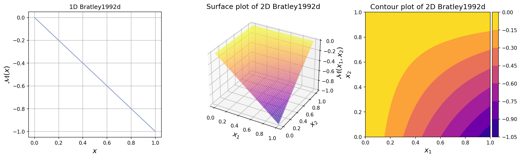
The plots for one-dimensional and two-dimensional Bratley1992d functions
are shown below.
Test function instance#
To create a default instance of the test function:
my_testfun = uqtf.Bratley1992d()
Check if it has been correctly instantiated:
print(my_testfun)
Function ID      : Bratley1992d
Input Dimension  : 2 (variable)
Output Dimension : 1
Parameterized    : False
Description      : Integration test function #4 from Bratley et al. (1992)
Applications     : integration, sensitivity
By default, the input dimension is set to \(2\)[1].
To create an instance with another value of input dimension,
pass an integer to the parameter input_dimension (keyword only).
For example, to create an instance of 10-dimensional Bratley1992d function,
type:
my_testfun = uqtf.Bratley1992d(input_dimension=10)
Description#
The Bratley1992d function is defined as follows[2]:
where \(\boldsymbol{x} = \{ x_1, \ldots, x_M \}\) is the \(M\)-dimensional vector of input variables further defined below.
Probabilistic input#
Based on [BFN92], the test function is integrated over the hypercube domain of \([0, 1]^M\). This specification was adopted in the application of the function as global sensitivity analysis test functions (see [SAA+10, KRFPS09]).
Such an input specification can be modeled using an \(M\) independent uniform random variables as shown in the table below.
No. |
Name |
Distribution |
Parameters |
Description |
|---|---|---|---|---|
1 |
\(x_1\) |
uniform |
[0.0 1.0] |
N/A |
\(\vdots\) |
\(\vdots\) |
\(\vdots\) |
\(\vdots\) |
\(\vdots\) |
M |
\(x_M\) |
uniform |
[0.0 1.0] |
N/A |
Reference results#
This section provides several reference results of typical UQ analyses involving the test function.
Definite integration#
The integral value of the function over the domain of \([0.0, 1.0]^M\) is analytical:
Moments#
The moments of the test function are analytically known and the first two moments are given below.
Expected value#
Due to the domain being a hypercube, the above integral value over the domain is the same as the expected value:
Variance#
The analytical value for the variance [SAA+10] is given as:
Sensitivity analysis#
Some sensitivity measures of the test function are known analytically; they make the function ideal for testing sensitivity analysis methods.
Total-effect Sobol’ indices#
The total-effect Sobol’ indices for the input variable \(m\) is given below as a function of the total number of dimensions \(M\):
where:
\(\mathbb{E}[\mathcal{M}^2](M) = \frac{1}{6} \left( 1 - \left( \frac{1}{3} \right)^M \right) + \frac{4}{15} \left( (-1)^{M+1} \left( \frac{1}{2} \right)^M + \left(\frac{1}{3} \right)^M \right)\)
\(E(m) = \frac{1}{6} \left( 1 - \left( \frac{1}{3} \right)^{m-1} \right) + \frac{4}{15} \left( (-1)^{m} \left( \frac{1}{2} \right)^{m-1} + \left(\frac{1}{3} \right)^{m-1} \right)\)
\(T_1(m, M) = \frac{1}{2} \left( \frac{1}{3} \right)^{m-2} \left( 1 - \left( \frac{1}{3} \right)^{M - m + 1} \right)\)
\(T_2(m, M) = \frac{1}{2} \left( \left( \frac{1}{3} \right)^{m-1} - \left( \frac{1}{3} \right)^M \right)\)
\(T_3(m, M) = \frac{3}{5} \left( 4 \left( \frac{1}{3} \right)^{M+1} + (-1)^{m+M} \left( \frac{1}{2} \right)^{M - m - 1} \left( \frac{1}{3} \right)^m \right)\)
\(T_4(m, M) = \frac{1}{5} \left( (-1)^{m+1} \left( \frac{1}{3} \right) \left( \frac{1}{2} \right)^{m - 3} - 4 \left( \frac{1}{3} \right)^m \right)\)
\(T_5(m, M) = \frac{1}{5} \left( (-1)^{M+1} \left( \frac{1}{3} \right) \left( \frac{1}{2} \right)^{M-2} + (-1)^{M + m - 1} \left( \frac{1}{3} \right)^m \left( \frac{1}{2} \right)^{M - m - 1} \right)\)
\(\mathbb{V}[\mathcal{M}](M)\) is the variance of the function as given in the previous section.
References#
Andrea Saltelli, Paola Annoni, Ivano Azzini, Francesca Campolongo, Marco Ratto, and Stefano Tarantola. Variance based sensitivity analysis of model output. design and estimator for the total sensitivity index. Computer Physics Communications, 181(2):259–270, 2010. doi:10.1016/j.cpc.2009.09.018.
Paul Bratley, Bennett L. Fox, and Harald Niederreiter. Implementation and tests of low-discrepancy sequences. ACM Transactions on Modeling and Computer Simulation, 2(3):195–213, 1992. doi:10.1145/146382.146385.
S. Kucherenko, M. Rodriguez-Fernandez, C. Pantelides, and N. Shah. Monte Carlo evaluation of derivative-based global sensitivity measures. Reliability Engineering & System Safety, 94(7):1135–1148, 2009. doi:10.1016/j.ress.2008.05.006.