Undamped Oscillator

import numpy as np
import matplotlib.pyplot as plt
import uqtestfuns as uqtf

The undamped oscillator function (UndampedOscillator) is a six-dimensional, scalar-valued test function that models a non-linear, undamped, single-degree-of-freedom, forced oscillating mechanical system.

This function is frequently used as a test function for reliability analysis methods (see [RE93, SG05, EGL11, EGLR13, BB90, GBL03]). Additionally, in [LMS21], the function is employed as a test function for metamodeling exercises.

Test function instance

To create a default instance of the test function:

my_testfun = uqtf.UndampedOscillator()

Check if it has been correctly instantiated:

print(my_testfun)

Function ID      : UndampedOscillator
Input Dimension  : 6 (fixed)
Output Dimension : 1
Parameterized    : False
Description      : Undamped, non-linear, single DOF oscillator
Applications     : reliability, metamodeling

Description

The system under consideration is a single-degree-of-freedom mechanical system that undergoes undamped forced oscillation. The performance function is analytically defined as follows[1]:

\[ g(\boldsymbol{x}) = 3 r - \lvert z_{\text{max}} \rvert, \]

where \(z_{\text{max}}\) is the maximum displacement response of the system given by

\[ z_{\text{max}} (\boldsymbol{x}) = \frac{2 F_1}{m \omega_0^2} \sin{\left( \frac{\omega_0 t_1}{2} \right)} \]

and

\[ \omega_0 = \sqrt{\frac{c_1 + c_2}{m}}. \]

\(\boldsymbol{x} = \{ m, c_1, c_2, r, F_1, t_1 \}\) is the six-dimensional vector of input variables probabilistically defined further below.

The failure state and the failure probability are defined as \(g(\boldsymbol{x}; \boldsymbol{p}) \leq 0\) and \(\mathbb{P}[g(\boldsymbol{X}; \boldsymbol{p}) \leq 0]\), respectively.

Probabilistic input

The available probabilistic input models are shown in the table below. The different specifications alter the failure probability of the system (as expected).

Table 10 Available probabilistic input of the undamped oscillator function

No.	Remark	Keyword	Source
1.	\(\mu_{F_1} = 1.00\)	Gayton2003 (default)	[GBL03] (Table 9)
2.	\(\mu_{F_1} = 0.60\)	Echard2013-1	[EGLR13] (Table 4)
3.	\(\mu_{F_1} = 0.45\)	Echard2013-2	[EGLR13] (Table 4)

The default input is shown below.

Show code cell source Hide code cell source

print(my_testfun.prob_input)

Function ID     : UndampedOscillator
Input ID        : Gayton2003
Input Dimension : 6
Description     : Input model for the undamped non-linear oscillator from
                  Gayton et al. (2003) (Table 9)
Marginals       :

 No.    Name    Distribution    Parameters          Description
-----  ------  --------------  ------------  --------------------------
  1      m         normal      [1.   0.05]              Mass
  2      c1        normal       [1.  0.1]       Spring (1) constant
  3      c2        normal      [0.1  0.01]      Spring (2) constant
  4      r         normal      [0.5  0.05]   Length of restoring force
  5      F1        normal       [1.  0.2]            Pulse load
  6      t1        normal       [1.  0.2]    Duration of the pulse load

Copulas         : Independence

Reference results

This section provides several reference results of typical UQ analyses involving the test function.

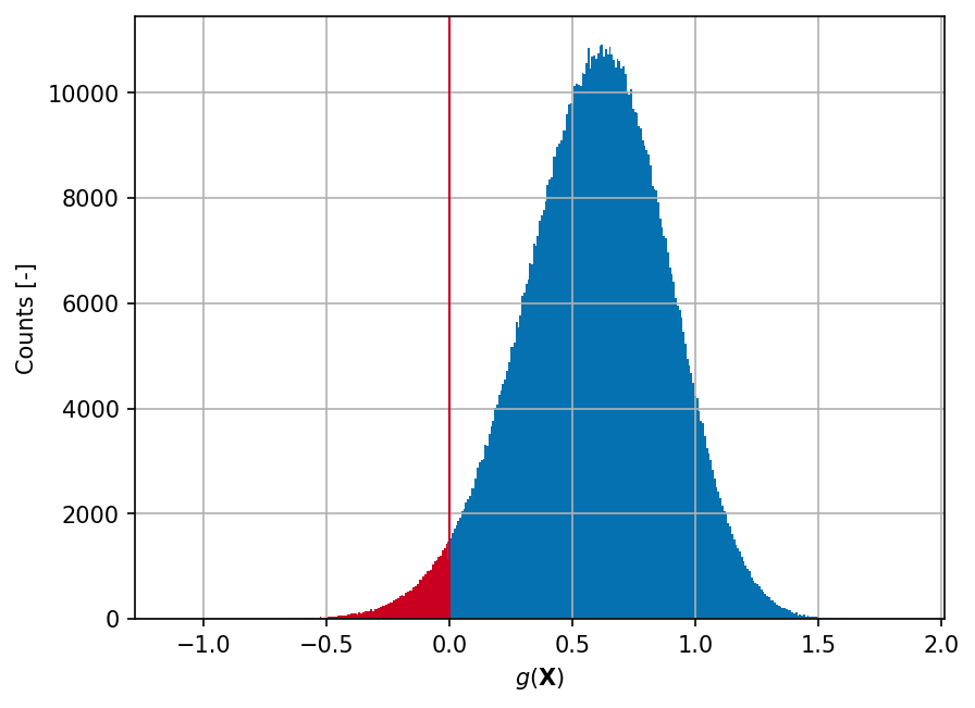
Sample histogram

Shown below is the histogram of the output based on \(10^6\) random points:

Show code cell source Hide code cell source

xx_test = my_testfun.prob_input.get_sample(1000000)
yy_test = my_testfun(xx_test)
idx_pos = yy_test > 0
idx_neg = yy_test <= 0

hist_pos = plt.hist(yy_test, bins="auto", color="#0571b0")
plt.hist(yy_test[idx_neg], bins=hist_pos[1], color="#ca0020")
plt.axvline(0, linewidth=1.0, color="#ca0020")

plt.grid()
plt.ylabel("Counts [-]")
plt.xlabel("$g(\mathbf{X})$")
plt.gcf().set_dpi(150);

Failure probability (\(P_f\))

Some reference values for the failure probability \(P_f\) from the literature are summarized in the tables below according to the chosen input specification.

Gayton2003

Method	\(N\)	\(\hat{P}_f\)	\(\mathrm{CoV}[\hat{P}_f]\)	Source
DS	\(1281\)	\(3.5 \times 10^{-2}\)	—	[SG05] (Table 5)
DS + Polynomial	\(62\)	\(3.4 \times 10^{-2}\)	—	[SG05] (Table 5)
DS + Splines	\(76\)	\(3.4 \times 10^{-2}\)	—	[SG05] (Table 5)
DS + Neural network (NN)	\(86\)	\(2.8 \times 10^{-2}\)	—	[SG05] (Table 5)
MCS + IS	\(6144\)	\(2.7 \times 10^{-2}\)	—	[SG05] (Table 5)
MCS + IS + Polynomials	\(109\)	\(2.5 \times 10^{-2}\)	—	[SG05] (Table 5)
MCS + IS + Splines	\(67\)	\(2.7 \times 10^{-2}\)	—	[SG05] (Table 5)
MCS + IS + NN	\(68\)	\(3.1 \times 10^{-2}\)	—	[SG05] (Table 5)
MCS	\(7 \times 10^{4}\)	\(2.834 \times 10^{-2}\)	\(2.2\%\)	[EGL11] (Table 6)
Adaptive Kriging + MCS + EFF	\(58\)	\(2.834 \times 10^{-2}\)	—	[EGL11] (Table 6)
Adaptive Kriging + MCS + U	\(45\)	\(2.851 \times 10^{-2}\)	—	[EGL11] (Table 6)

Echard2013-1

Method	\(N\)	\(\hat{P}_f\)	\(\mathrm{CoV}[\hat{P}_f]\)	Source
MCS	\(1.8 \times 10^{8}\)	\(9.09 \times 10^{-6}\)	\(2.47\%\)	[EGLR13] (Table 5)
FORM	\(29\)	\(9.76 \times 10^{-6}\)	—	[EGLR13] (Table 5)
IS	\(20 + \times 10^{4}\)	\(9.13 \times 10^{-6}\)	\(2.29\%\)	[EGLR13] (Table 5)
Adaptive Kriging + IS	\(29 + 38\)	\(9.13 \times 10^{-6}\)	\(2.29\%\)	[EGLR13] (Table 5)

Echard2013-2

Method	\(N\)	\(\hat{P}_f\)	\(\mathrm{CoV}[\hat{P}_f]\)	Source
MCS	\(9 \times 10^{8}\)	\(1.55 \times 10^{-8}\)	\(2.68\%\)	[EGLR13] (Table 5)
FORM	\(29\)	\(1.56 \times 10^{-8}\)	—	[EGLR13] (Table 5)
IS	\(29 + \times 10^{4}\)	\(1.53 \times 10^{-8}\)	\(2.70\%\)	[EGLR13] (Table 5)
Adaptive Kriging + IS	\(29 + 38\)	\(1.54 \times 10^{-8}\)	\(2.70\%\)	[EGLR13] (Table 5)

References

[RE93]

Malur R. Rajashekhar and Bruce R. Ellingwood. A new look at the response surface approach for reliability analysis. Structural Safety, 12(3):205–220, 1993. doi:10.1016/0167-4730(93)90003-j.

[SG05] (1,2,3,4,5,6,7,8,9)

Luc Schueremans and Dionys Van Gemert. Benefit of splines and neural networks in simulation based structural reliability analysis. Structural Safety, 27(3):246–261, 2005. doi:10.1016/j.strusafe.2004.11.001.

[EGL11] (1,2,3,4)

B. Echard, N. Gayton, and M. Lemaire. AK-MCS: an active learning reliability method combining kriging and Monte Carlo simulation. Structural Safety, 33(2):145–154, 2011. doi:10.1016/j.strusafe.2011.01.002.

[EGLR13] (1,2,3,4,5,6,7,8,9,10,11)

B. Echard, N. Gayton, M. Lemaire, and N. Relun. A combined importance sampling and kriging reliability method for small failure probabilities with time-demanding numerical models. Reliability Engineering & System Safety, 111:232–240, 2013. doi:10.1016/j.ress.2012.10.008.

[BB90]

C. G. Bucher and U. Bourgund. A fast and efficient response surface approach for structural reliability problems. Structural Safety, 7(1):57–66, 1990. doi:10.1016/0167-4730(90)90012-e.

[GBL03] (1,2,3)

N. Gayton, J. M. Bourinet, and M. Lemaire. CQ2RS: a new statistical approach to the response surface method for reliability analysis. Structural Safety, 25(1):99–121, 2003. doi:10.1016/s0167-4730(02)00045-0.

[LMS21]

Nora Lüthen, Stefano Marelli, and Bruno Sudret. Sparse polynomial chaos expansions: literature survey and benchmark. SIAM/ASA Journal on Uncertainty Quantification, 9(2):593–649, 2021. doi:10.1137/20m1315774.

---

[1]

see Section 6.4.1 in [GBL03].