Oakley and O’Hagan (2002) One-dimensional (1D) Function

The 1D function from Oakley and O’Hagan (2002) (or Oakley1D function for short) is a scalar-valued test function. It was used in [OOHagan02] as a test function for illustrating metamodeling and uncertainty propagation approaches.

import numpy as np
import matplotlib.pyplot as plt
import uqtestfuns as uqtf

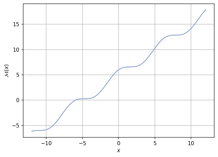
A plot of the function is shown below for \(x \in [-12, 12]\).

Test function instance

To create a default instance of the test function:

my_testfun = uqtf.Oakley1D()

Check if it has been correctly instantiated:

print(my_testfun)

Function ID      : Oakley1D
Input Dimension  : 1 (fixed)
Output Dimension : 1
Parameterized    : False
Description      : One-dimensional function from Oakley and O'Hagan (2002)
Applications     : metamodeling

Description

The test function is analytically defined as follows:

\[ \mathcal{M}(x) = 5 + x + \cos{x}, \]

where \(x\) is probabilistically defined below.

Probabilistic input

Based on [OOHagan02], the probabilistic input model for the 1D Oakley-O’Hagan function consists of a normal random variable with the parameters shown in the table below.

Show code cell source Hide code cell source

print(my_testfun.prob_input)

Function ID     : Oakley1D
Input ID        : Oakley2002
Input Dimension : 1
Description     : Probabilistic input model for the one-dimensional
                  function from Oakley and O'Hagan (2002)
Marginals       :

 No.    Name    Distribution    Parameters    Description
-----  ------  --------------  ------------  -------------
  1      x         normal        [0. 4.]           -

Reference results

This section provides several reference results of typical UQ analyses involving the test function.

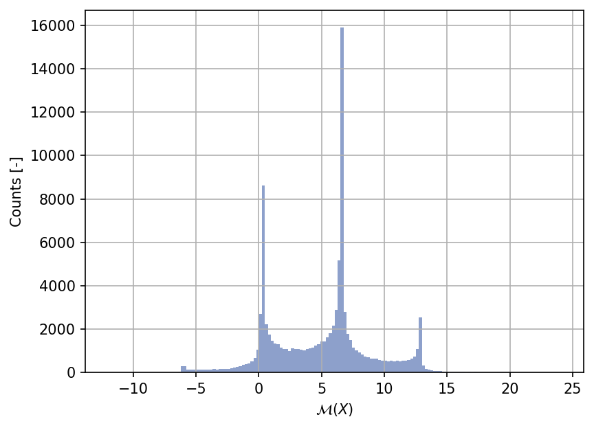
Sample histogram

Shown below is the histogram of the output based on \(100'000\) random points:

Show code cell source Hide code cell source

np.random.seed(42)
xx_test = my_testfun.prob_input.get_sample(100000)
yy_test = my_testfun(xx_test)

plt.hist(yy_test, bins="auto", color="#8da0cb");
plt.grid();
plt.ylabel("Counts [-]");
plt.xlabel("$\mathcal{M}(X)$");
plt.gcf().tight_layout(pad=3.0)
plt.gcf().set_dpi(150);

Moment estimations

Shown below is the convergence of a direct Monte-Carlo estimation of the output mean and variance with increasing sample sizes.

Show code cell source Hide code cell source

np.random.seed(42)
sample_sizes = np.array([1e1, 1e2, 1e3, 1e4, 1e5, 1e6], dtype=int)
mean_estimates = np.empty((len(sample_sizes), 50))
var_estimates = np.empty((len(sample_sizes), 50))

for i, sample_size in enumerate(sample_sizes):
    for j in range(50):
        xx_test = my_testfun.prob_input.get_sample(sample_size)
        yy_test = my_testfun(xx_test)
        mean_estimates[i, j] = np.mean(yy_test)
        var_estimates[i, j] = np.var(yy_test)

# --- Compute the error associated with the estimates
mean_estimates_errors = np.std(mean_estimates, axis=1)
var_estimates_errors = np.std(var_estimates, axis=1)

# --- Plot the mean and variance estimates
fig, ax_1 = plt.subplots(figsize=(6,4))

# --- Mean plot
ax_1.errorbar(
    sample_sizes,
    mean_estimates[:,0],
    yerr=2.0*mean_estimates_errors,
    marker="o",
    color="#66c2a5",
    label="Mean"
)
ax_1.set_xlim([5, 2e6])
ax_1.set_xlabel("Sample size")
ax_1.set_ylabel("Output mean estimate")
ax_1.set_xscale("log");
ax_2 = ax_1.twinx()

# --- Variance plot
ax_2.errorbar(
    sample_sizes+1,
    var_estimates[:,0],
    yerr=1.96*var_estimates_errors,
    marker="o",
    color="#fc8d62",
    label="Variance",
)
ax_2.set_ylabel("Output variance estimate")

# Add the two plots together to have a common legend
ln_1, labels_1 = ax_1.get_legend_handles_labels()
ln_2, labels_2 = ax_2.get_legend_handles_labels()
ax_2.legend(ln_1 + ln_2, labels_1 + labels_2, loc=0)

plt.grid()
fig.set_dpi(150)

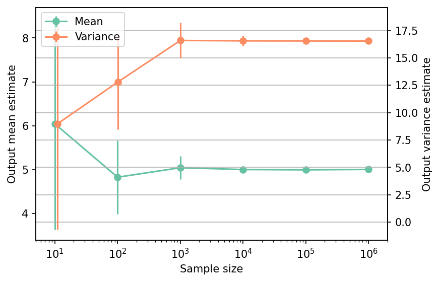
The tabulated results for each sample size is shown below.

Show code cell source Hide code cell source

from tabulate import tabulate

# --- Compile data row-wise
outputs =[]

for (
    sample_size,
    mean_estimate,
    mean_estimate_error,
    var_estimate,
    var_estimate_error,
) in zip(
    sample_sizes,
    mean_estimates[:,0],
    2.0*mean_estimates_errors,
    var_estimates[:,0],
    2.0*var_estimates_errors,
):
    outputs += [
        [
            sample_size,
            mean_estimate,
            mean_estimate_error,
            var_estimate,
            var_estimate_error,
            "Monte-Carlo",
        ],
    ]

header_names = [
    "Sample size",
    "Mean",
    "Mean error",
    "Variance",
    "Variance error",
    "Remark",
]

tabulate(
    outputs,
    numalign="center",
    stralign="center",
    tablefmt="html",
    floatfmt=(".1e", ".4e", ".4e", ".4e", ".4e", "s"),
    headers=header_names
)

Sample size	Mean	Mean error	Variance	Variance error	Remark
1.0e+01	6.0420e+00	2.4129e+00	8.9813e+00	9.8511e+00	Monte-Carlo
1.0e+02	4.8235e+00	8.4273e-01	1.2799e+01	4.4187e+00	Monte-Carlo
1.0e+03	5.0407e+00	2.6215e-01	1.6591e+01	1.6444e+00	Monte-Carlo
1.0e+04	4.9989e+00	7.2706e-02	1.6555e+01	4.7489e-01	Monte-Carlo
1.0e+05	4.9918e+00	2.5262e-02	1.6546e+01	1.4939e-01	Monte-Carlo
1.0e+06	5.0017e+00	7.9593e-03	1.6540e+01	4.5595e-02	Monte-Carlo

References

[OOHagan02] (1,2)

Jeremy Oakley and Anthony O'Hagan. Bayesian inference for the uncertainty distribution of computer model outputs. Biometrika, 89(4):769–784, 2002. doi:10.1093/biomet/89.4.769.