Two-dimensional Function from Cheng and Sandu (2010)#
import numpy as np
import matplotlib.pyplot as plt
import uqtestfuns as uqtf
The two-dimensional test function from Cheng and Sandu (2002) (or
Cheng2D for short) is used in a metamodeling exercise via polynomial
chaos expansion in [CS10].
Test function instance#
To create a default instance of the test function:
my_testfun = uqtf.Cheng2D()
Check if it has been correctly instantiated:
print(my_testfun)
Function ID      : Cheng2D
Input Dimension  : 2 (fixed)
Output Dimension : 1
Parameterized    : False
Description      : Two-dimensional test function from Cheng and Sandu (2010)
Applications     : metamodeling
Description#
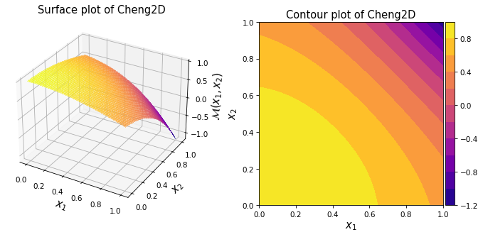
The test function is defined as follows[1]:
where \(\boldsymbol{x} = \{ x_1, x_2 \}\) is the two-dimensional vector of input variables further defined below.
Probabilistic input#
The input consists of two uniformly distributed random variables as shown below.
Show code cell source
print(my_testfun.prob_input)
Function ID     : Cheng2D
Input ID        : Cheng2010
Input Dimension : 2
Description     : Probabilistic input model for the 2D test function from
                  Cheng and Sandu (2010)
Marginals       :

 No.    Name    Distribution    Parameters    Description
-----  ------  --------------  ------------  -------------
  1      X1       uniform        [0. 1.]           -
  2      X2       uniform        [0. 1.]           -

Copulas         : Independence
Reference results#
This section provides several reference results of typical UQ analyses involving the test function.
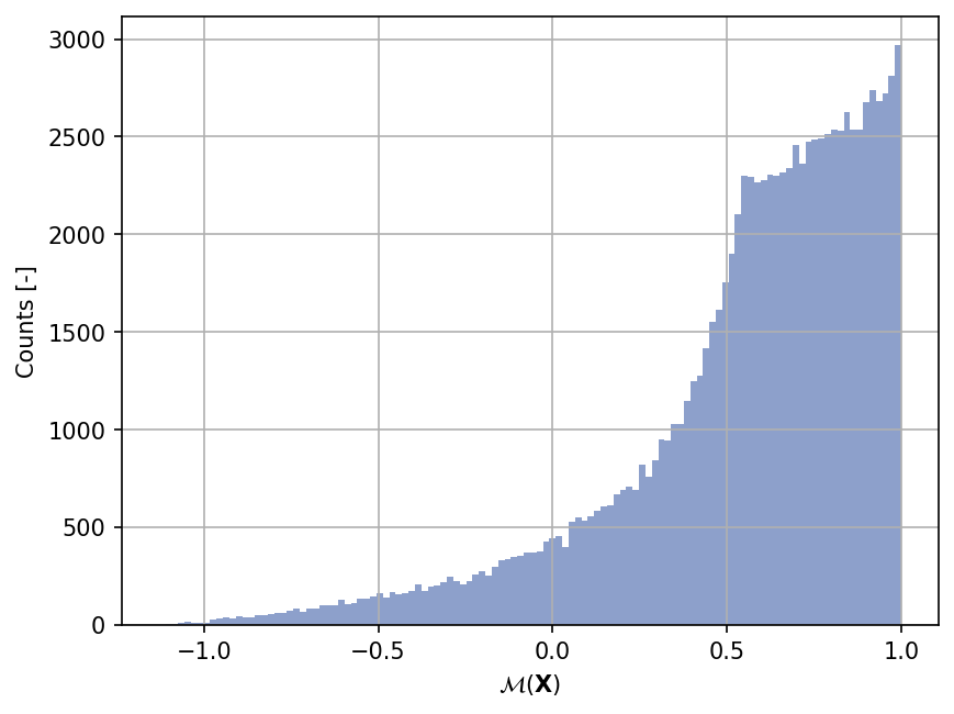
Sample histogram#
Shown below is the histogram of the output based on \(100'000\) random points:
Show code cell source
xx_test = my_testfun.prob_input.get_sample(100000)
yy_test = my_testfun(xx_test)

plt.hist(yy_test, bins="auto", color="#8da0cb");
plt.grid();
plt.ylabel("Counts [-]");
plt.xlabel("$\mathcal{M}(\mathbf{X})$");
plt.gcf().set_dpi(150);
References#
Haiyan Cheng and Adrian Sandu. Collocation least-squares polynomial chaos method. In Proceedings of the 2010 Spring Simulation Multiconference, SpringSim ’10, 1–6. Society for Computer Simulation International, 2010. doi:10.1145/1878537.1878621.