Saltelli Linear Function

The Saltelli Linear function is an \(M\)-dimensional scalar-valued function. It was introduced in [SCS08] for illustrating sensitivity analysis methods. It is later used in [SCJR22] for benchmarking various sensitivity analysis methods.

Due to its simple form, the moments and Sobol’ sensitivity indices may be computed analytically.

import numpy as np
import matplotlib.pyplot as plt
import uqtestfuns as uqtf

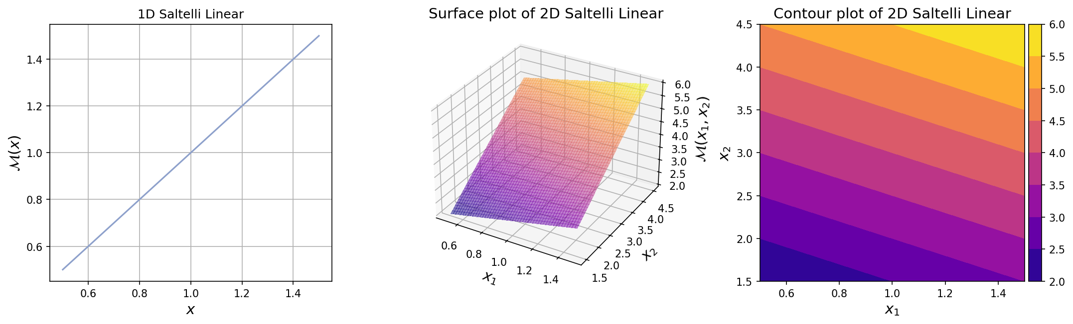
The plots for one-dimensional and two-dimensional Sobol’-G function can be seen below.

Test function instance

To create a default instance of the test function, type:

my_testfun = uqtf.SaltelliLinear()

Check if it has been correctly instantiated:

print(my_testfun)

Function ID      : SaltelliLinear
Input Dimension  : 2 (variable)
Output Dimension : 1
Parameterized    : False
Description      : Linear function from Saltelli et al. (2000)
Applications     : sensitivity

By default, the input dimension is set to \(2\)[1]. To create an instance with another value of input dimension, pass an integer to the parameter input_dimension (the first parameter). For example, to create an instance of the Saltelli Linear function in six dimensions, type:

my_testfun = uqtf.SaltelliLinear(input_dimension=6)

In the subsequent section, the function will be illustrated using six dimensions.

Description

The Saltelli Linear function is defined as follows:

\[ \mathcal{M}(\boldsymbol{x}) = \sum_{i = 1}^M x_i \]

where \(\boldsymbol{x} = \{ x_1, \ldots, x_M \}\) is the \(M\)-dimensional vector of input variables further defined below.

Probabilistic input

Based on [SCS08] the probabilistic input model for the function consists of \(M\) independent uniform random variables with the following ranges:

\[ X_i \sim \mathcal{U}[x_{o, i} - \sigma_{o, i}, x_{o, i} + \sigma_{o, i}], \; i = 1, \ldots, M, \]

where \(x_{o, i} = 3^{i - 1}\) and \(\sigma_{o, i} = 0.5 * x_{o, i}\). Notice that the higher the variable index, the larger its uncertainty both in absolute sense (i.e., the standard deviation is larger) and in relative sense (i.e., the coefficient of variation is larger).

For the six-variable model, the ranges are shown below.

Show code cell source Hide code cell source

print(my_testfun.prob_input)

Function ID     : SaltelliLinear
Input ID        : Saltelli2000
Input Dimension : 6
Description     : Probabilistic input model for the linear function from
                  Saltelli et al. (2000)
Marginals       :

 No.    Name    Distribution    Parameters     Description
-----  ------  --------------  -------------  -------------
  1      X1       uniform        [0.5 1.5]          -
  2      X2       uniform        [1.5 4.5]          -
  3      X3       uniform       [ 4.5 13.5]         -
  4      X4       uniform       [13.5 40.5]         -
  5      X5       uniform      [ 40.5 121.5]        -
  6      X6       uniform      [121.5 364.5]        -

Copulas         : Independence

Reference results

This section provides several reference results of typical UQ analyses involving the test function.

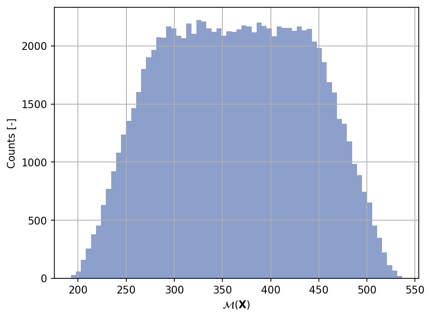
Sample histogram

Shown below is the histogram of the output based on \(100'000\) random points:

Show code cell source Hide code cell source

my_testfun.prob_input.reset_rng(42)
xx_test = my_testfun.prob_input.get_sample(100000)
yy_test = my_testfun(xx_test)

plt.hist(yy_test, bins="auto", color="#8da0cb");
plt.grid();
plt.ylabel("Counts [-]");
plt.xlabel("$\mathcal{M}(\mathbf{X})$");
plt.gcf().set_dpi(150);

Moments estimation

The mean and variance of the Sobol’-G function can be computed analytically.

The mean is given as follows:

\[ \mathbb{E}[Y] = \sum_{i = 1}^M \mathbb{E}[X_i] = \sum_{i = 1}^M x_{o, i}, \]

where \(x_{o, i} = 3^{i - 1}, i = 1, \ldots, M\).

The variance is given as follows:

\[ \mathbb{V}[Y] = \sum_{i = 1}^M \mathbb{V}[X_i] = \frac{1}{12} \sum_{i = 1}^M x_{o, i}^2, \]

The means and variances for the linear function up to dimension \(10\) are shown in the table below.

Show code cell source Hide code cell source

from tabulate import tabulate

input_dims = 10

# --- Compile data row-wise

outputs = []
for input_dim in range(1, input_dims + 1):
    xx_o = 3**(np.arange(1, input_dim + 1) - 1)
    outputs.append(
        [input_dim, np.sum(xx_o), np.sum(xx_o**2) / 12]
    )

header_names = [
    "Input dimensions",
    "Mean",
    "Variance",
]

tabulate(
    outputs,
    numalign="center",
    stralign="center",
    tablefmt="html",
    floatfmt=("d", ".4e", ".4e"),
    headers=header_names
)

Input dimensions	Mean	Variance
1	1.0000e+00	8.3333e-02
2	4.0000e+00	8.3333e-01
3	1.3000e+01	7.5833e+00
4	4.0000e+01	6.8333e+01
5	1.2100e+02	6.1508e+02
6	3.6400e+02	5.5358e+03
7	1.0930e+03	4.9823e+04
8	3.2800e+03	4.4840e+05
9	9.8410e+03	4.0356e+06
10	2.9524e+04	3.6321e+07

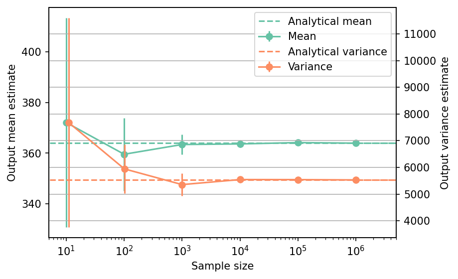
Shown below is the convergence of a direct Monte-Carlo estimation of the output mean and variance with increasing sample sizes compared with the analytical values. The error bars correspond to twice the standard deviation of the estimates obtained from \(50\) replications.

Show code cell source Hide code cell source

# --- Compute the mean and variance estimate
my_testfun.prob_input.reset_rng(42)
sample_sizes = np.array([1e1, 1e2, 1e3, 1e4, 1e5, 1e6], dtype=int)
mean_estimates = np.empty((len(sample_sizes), 50))
var_estimates = np.empty((len(sample_sizes), 50))

for i, sample_size in enumerate(sample_sizes):
    for j in range(50):
        xx_test = my_testfun.prob_input.get_sample(sample_size)
        yy_test = my_testfun(xx_test)
        mean_estimates[i, j] = np.mean(yy_test)
        var_estimates[i, j] = np.var(yy_test)

mean_estimates_errors = np.std(mean_estimates, axis=1)
var_estimates_errors = np.std(var_estimates, axis=1)

# --- Compute analytical mean and variance
xx_o = 3**(np.arange(1, my_testfun.input_dimension + 1) - 1)
mean_analytical = np.sum(xx_o)
var_analytical = np.sum(xx_o**2) / 12.0

# --- Plot the mean and variance estimates
fig, ax_1 = plt.subplots(figsize=(6,4))

ext_sample_sizes = np.insert(sample_sizes, 0, 1)
ext_sample_sizes = np.insert(ext_sample_sizes, -1, 5e6)

# --- Mean plot
ax_1.errorbar(
    sample_sizes,
    mean_estimates[:,0],
    yerr=2.0*mean_estimates_errors,
    marker="o",
    color="#66c2a5",
    label="Mean"
)
# Plot the analytical mean
ax_1.plot(
    ext_sample_sizes,
    np.repeat(mean_analytical, len(ext_sample_sizes)),
    linestyle="--",
    color="#66c2a5",
    label="Analytical mean",
)
ax_1.set_xlim([5, 5e6])
ax_1.set_xlabel("Sample size")
ax_1.set_ylabel("Output mean estimate")
ax_1.set_xscale("log");
ax_2 = ax_1.twinx()

# --- Variance plot
ax_2.errorbar(
    sample_sizes+1,
    var_estimates[:,0],
    yerr=2.0*var_estimates_errors,
    marker="o",
    color="#fc8d62",
    label="Variance",
)
# Plot the analytical variance
ax_2.plot(
    ext_sample_sizes,
    np.repeat(var_analytical, len(ext_sample_sizes)),
    linestyle="--",
    color="#fc8d62",
    label="Analytical variance",
)
ax_2.set_ylabel("Output variance estimate")

# Add the two plots together to have a common legend
ln_1, labels_1 = ax_1.get_legend_handles_labels()
ln_2, labels_2 = ax_2.get_legend_handles_labels()
ax_2.legend(ln_1 + ln_2, labels_1 + labels_2, loc=0)

plt.grid()
fig.set_dpi(150)

The tabulated results for each sample size is shown below.

Show code cell source Hide code cell source

from tabulate import tabulate

# --- Compile data row-wise
outputs = [
    [
        np.nan,
        mean_analytical,
        0.0,
        var_analytical,
        0.0,
        "Analytical",
    ]
]

for (
    sample_size,
    mean_estimate,
    mean_estimate_error,
    var_estimate,
    var_estimate_error,
) in zip(
    sample_sizes,
    mean_estimates[:,0],
    2.0*mean_estimates_errors,
    var_estimates[:,0],
    2.0*var_estimates_errors,
):
    outputs += [
        [
            sample_size,
            mean_estimate,
            mean_estimate_error,
            var_estimate,
            var_estimate_error,
            "Monte-Carlo",
        ],
    ]

header_names = [
    "Sample size",
    "Mean",
    "Mean error",
    "Variance",
    "Variance error",
    "Remark",
]

tabulate(
    outputs,
    numalign="center",
    stralign="center",
    tablefmt="html",
    floatfmt=(".1e", ".4e", ".4e", ".4e", ".4e", "s"),
    headers=header_names
)

Sample size	Mean	Mean error	Variance	Variance error	Remark
nan	3.6400e+02	0.0000e+00	5.5358e+03	0.0000e+00	Analytical
1.0e+01	3.7212e+02	4.1366e+01	7.6812e+03	3.9197e+03	Monte-Carlo
1.0e+02	3.5956e+02	1.4402e+01	5.9433e+03	9.1394e+02	Monte-Carlo
1.0e+03	3.6341e+02	3.9072e+00	5.3550e+03	4.1784e+02	Monte-Carlo
1.0e+04	3.6365e+02	1.4752e+00	5.5438e+03	1.2694e+02	Monte-Carlo
1.0e+05	3.6418e+02	4.5023e-01	5.5415e+03	3.9981e+01	Monte-Carlo
1.0e+06	3.6395e+02	1.4023e-01	5.5294e+03	1.0097e+01	Monte-Carlo

Sensitivity indices

The main-effect Sobol’ sensitivity indices of the linear function are given by the following formula:

\[ S_i \equiv \frac{V_i}{\mathbb{V}[Y]} = \frac{\mathbb{V}[X_i]}{\mathbb{V}[Y]} = \frac{x_{o, i}^2}{\sum_{i = 1}^M x_{o, i}^2},\; i = 1, \ldots, M. \]

Since there is no interaction effect present in the model, the total-effect indices are equal to the main-effect indices.

Some example values of the main-effect indices for the linear function up to dimension \(6\) is shown in the table below.

Show code cell source Hide code cell source

from tabulate import tabulate

input_dims = 6

# --- Compile data row-wise

outputs = []
for input_dim in range(input_dims):
    output = [f"X{input_dim + 1}"]
    for _ in range(input_dim):
        output.append(0.0)
    for i in range(input_dim, input_dims):
        xx_o = 3**(np.arange(1, i + 2) - 1)
        
        output.append(
            xx_o[input_dim]**2 / np.sum(xx_o**2)
        )

    outputs.append(output)

header_names = [
    "Si",
    "m = 1",
    "m = 2",
    "m = 3",
    "m = 4",
    "m = 5",
    "m = 6",
]

tabulate(
    outputs,
    numalign="center",
    stralign="center",
    tablefmt="html",
    floatfmt=("s", ".4e", ".4e", ".4e", ".4e", ".4e", ".4e"),
    headers=header_names
)

Si	m = 1	m = 2	m = 3	m = 4	m = 5	m = 6
X1	1.0000e+00	1.0000e-01	1.0989e-02	1.2195e-03	1.3548e-04	1.5053e-05
X2	0.0000e+00	9.0000e-01	9.8901e-02	1.0976e-02	1.2193e-03	1.3548e-04
X3	0.0000e+00	0.0000e+00	8.9011e-01	9.8780e-02	1.0974e-02	1.2193e-03
X4	0.0000e+00	0.0000e+00	0.0000e+00	8.8902e-01	9.8767e-02	1.0974e-02
X5	0.0000e+00	0.0000e+00	0.0000e+00	0.0000e+00	8.8890e-01	9.8766e-02
X6	0.0000e+00	0.0000e+00	0.0000e+00	0.0000e+00	0.0000e+00	8.8889e-01

References

[SCJR22]

Xifu Sun, Barry Croke, Anthony Jakeman, and Stephen Roberts. Benchmarking Active Subspace methods of global sensitivity analysis against variance-based Sobol’ and Morris methods with established test functions. Environmental Modelling & Software, 149:105310, 2022. doi:10.1016/j.envsoft.2022.105310.

[SCS08] (1,2)

Andrea Saltelli, Karen Chan, and Evelyn Marian Scott, editors. Sensitivity analysis. Wiley Series in Probability and Statistics. John Wiley & Sons, Hoboken, NJ, 2008. ISBN 9780470743829.

---

[1]

This default dimension applies to all variable dimension test functions. It will be used if the input_dimension argument is not given.