Speed Reducer Shaft#
import numpy as np
import matplotlib.pyplot as plt
import uqtestfuns as uqtf
The speed reducer shaft test function is a five-dimensional scalar-valued test function introduced in [DS04]. It is used as a test function for reliability analysis algorithms (see, for instance, [LGG+18, DS04]).
Test function instance#
To create a default instance of the test function:
my_testfun = uqtf.SpeedReducerShaft()
Check if it has been correctly instantiated:
print(my_testfun)
Function ID      : SpeedReducerShaft
Input Dimension  : 5 (fixed)
Output Dimension : 1
Parameterized    : False
Description      : Reliability of a shaft in a speed reducer from Du and Sudjianto (2004)
Applications     : reliability
Description#
The function models the performance of a shaft in a speed reducer [DS04]. The performance is defined as the strength of the shaft subtracted by the stress as follows[1]:
where \(\boldsymbol{x} = \{ S, D, F, L, T \}\) is the five-dimensional vector of input variables probabilistically defined further below.
The failure event and the failure probability are defined as \(g(\boldsymbol{x}) \leq 0\) and \(\mathbb{P}[g(\boldsymbol{X}) \leq 0]\), respectively.
Probabilistic input#
Based on [DS04], the probabilistic input model for the speed reducer shaft reliability problem consists of five independent random variables with marginal distributions shown in the table below.
Show code cell source
print(my_testfun.prob_input)
Function ID     : SpeedReducerShaft
Input ID        : Du2004
Input Dimension : 5
Description     : Input model for the speed reducer shaft problem from Du
                  and Sudjianto (2004)
Marginals       :

 No.    Name    Distribution            Parameters                Description
-----  ------  --------------  -----------------------------  -------------------
  1      D         normal               [39.   0.1]           Shaft diameter [mm]
  2      L         normal             [4.e+02 1.e-01]           Shaft span [mm]
  3      F         gumbel      [1342.48137736  272.89388043]  External force [N]
  4      T         normal                [250  35]                Torque [Nm]
  5      S        uniform                 [70 80]               Strength [MPa]

Copulas         : Independence
Note that the variables \(F\), \(D\), and \(L\) must be first converted to their corresponding SI units (i.e., \([\mathrm{Pa}]\), \([\mathrm{m}]\), and \([\mathrm{m}]\), respectively) before the values are plugged into the formula above.
Reference results#
This section provides several reference results of typical UQ analyses involving the test function.
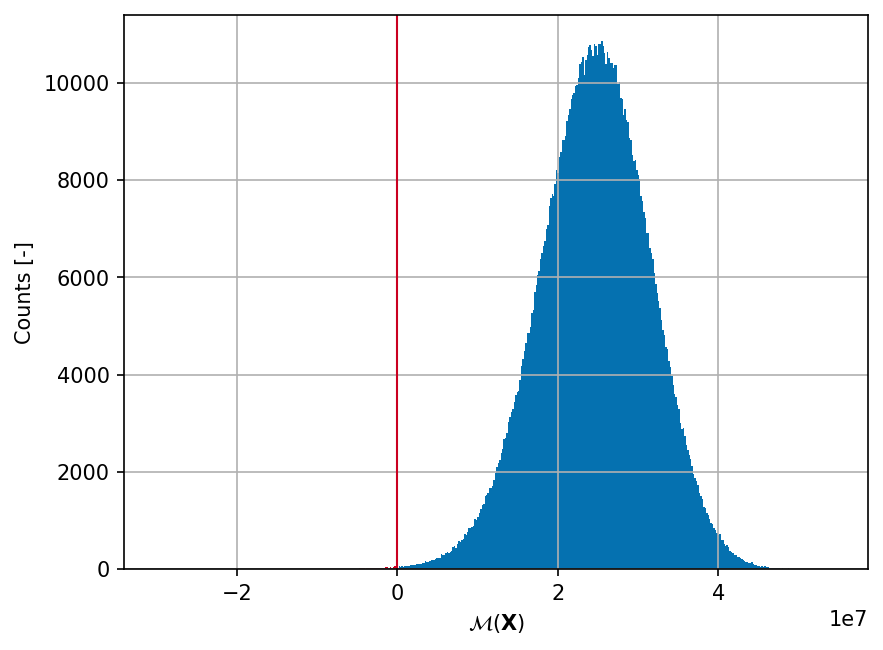
Sample histogram#
Shown below is the histogram of the output based on \(10^6\) random points:
Show code cell source
xx_test = my_testfun.prob_input.get_sample(1000000)
yy_test = my_testfun(xx_test)
idx_pos = yy_test > 0
idx_neg = yy_test <= 0

hist_pos = plt.hist(yy_test, bins="auto", color="#0571b0")
plt.hist(yy_test[idx_neg], bins=hist_pos[1], color="#ca0020")
plt.axvline(0, linewidth=1.0, color="#ca0020")

plt.grid()
plt.ylabel("Counts [-]")
plt.xlabel("$\mathcal{M}(\mathbf{X})$")
plt.gcf().set_dpi(150);
Failure probability#
Some reference values for the failure probability \(P_f\) and from the literature are summarized in the table below.
References#
Xu Li, Chunlin Gong, Liangxian Gu, Wenkun Gao, Zhao Jing, and Hua Su. A sequential surrogate method for reliability analysis based on radial basis function. Structural Safety, 73:42–53, 2018. doi:10.1016/j.strusafe.2018.02.005.