Flood Model

import numpy as np
import matplotlib.pyplot as plt
import uqtestfuns as uqtf

The flood model is an eight-dimensional scalar valued function. The model was used in the context of sensitivity analysis in [IL15, LIPG13] and has become a canonical example of the OpenTURNS package [BDIP17].

Test function instance

To create a default instance of the flood model:

my_testfun = uqtf.Flood()

Check if it has been correctly instantiated:

print(my_testfun)

Function ID      : Flood
Input Dimension  : 8 (fixed)
Output Dimension : 1
Parameterized    : False
Description      : Flood model from Iooss and Lemaître (2015)
Applications     : metamodeling, sensitivity

Description

The flood model computes the maximum annual underflow of a river using the following analytical formula:

\[\begin{split} \begin{align} \mathcal{M}(\boldsymbol{x}) & = z_v + h - h_d - c_b\\ h & = \left[ \frac{q}{b k_s \left(\frac{z_m - z_v}{l} \right)^{0.5}} \right]^{0.6} \end{align} \end{split}\]

where \(\boldsymbol{x} = \{ q, k_s, z_v, z_m, h_d, c_b, l, b \}\) is the eight-dimensional vector of input variables further defined below. The output is given in \([\mathrm{m}]\). A negative value indicates that an overflow (flooding) occurs.

Note

Compared to the original function, this implementation inverted the sign of the output such that underflowing has a positive sign.

The model is based on a simplification of the one-dimensional hydro-dynamical equations of St. Venant under the assumption of uniform and constant flow rate and a large rectangular section.

Probabilistic input

Based on [IL15] (Table 4), the probabilistic input model for the flood model consists of eight independent random variables with marginals shown in the table below.

Show code cell source Hide code cell source

print(my_testfun.prob_input)

Function ID     : Flood
Input ID        : Iooss2015
Input Dimension : 8
Description     : Probabilistic input model for the Flood model from Iooss
                  and Lemaître (2015)
Marginals       :

 No.    Name    Distribution          Parameters                     Description
-----  ------  --------------  -------------------------  ---------------------------------
  1      Q      trunc-gumbel   [1013.  558.  500. 3000.]  Maximum annual flow rate [m^3/s]
  2      Ks     trunc-normal       [30.  8. 15. inf]      Strickler coefficient [m^(1/3)/s]
  3      Zv      triangular          [49. 51. 50.]           River downstream level [m]
  4      Zm      triangular          [54. 56. 55.]            River upstream level [m]
  5      Hd       uniform               [7. 9.]                    Dyke height [m]
  6      Cb      triangular        [55.  56.  55.5]                Bank level [m]
  7      L       triangular       [4990. 5010. 5000.]      Length of the river stretch [m]
  8      B       triangular        [295. 305. 300.]                River width [m]

Copulas         : Independence

Reference results

This section provides several reference results of typical UQ analyses involving the test function.

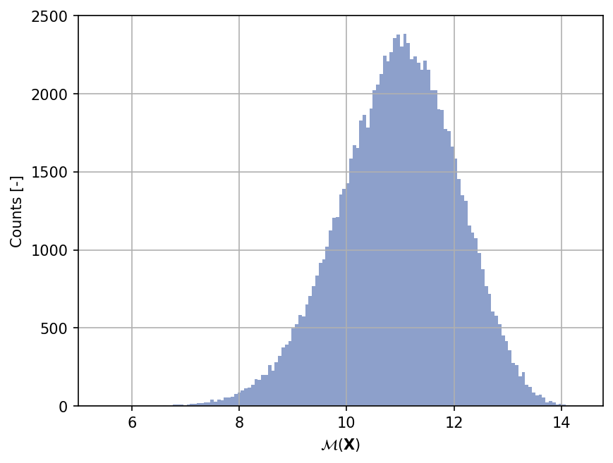
Sample histogram

Shown below is the histogram of the output based on \(100'000\) random points:

Show code cell source Hide code cell source

np.random.seed(42)
xx_test = my_testfun.prob_input.get_sample(100000)
yy_test = my_testfun(xx_test)

plt.hist(yy_test, bins="auto", color="#8da0cb");
plt.grid();
plt.ylabel("Counts [-]");
plt.xlabel("$\mathcal{M}(\mathbf{X})$");
plt.gcf().set_dpi(150);

Moments estimation

Shown below is the convergence of a direct Monte-Carlo estimation of the output mean and variance with increasing sample sizes.

Show code cell source Hide code cell source

# --- Compute the mean and variance estimate
np.random.seed(42)
sample_sizes = np.array([1e1, 1e2, 1e3, 1e4, 1e5, 1e6, 1e7], dtype=int)
mean_estimates = np.empty(len(sample_sizes))
var_estimates = np.empty(len(sample_sizes))

for i, sample_size in enumerate(sample_sizes):
    xx_test = my_testfun.prob_input.get_sample(sample_size)
    yy_test = my_testfun(xx_test)
    mean_estimates[i] = np.mean(yy_test)
    var_estimates[i] = np.var(yy_test)

# --- Compute the error associated with the estimates
mean_estimates_errors = np.sqrt(var_estimates) / np.sqrt(np.array(sample_sizes))
var_estimates_errors = var_estimates * np.sqrt(2 / (np.array(sample_sizes) - 1))

# --- Do the plot
fig, ax_1 = plt.subplots(figsize=(6,4))

ax_1.errorbar(
    sample_sizes,
    mean_estimates,
    yerr=mean_estimates_errors,
    marker="o",
    color="#66c2a5",
    label="Mean",
)
ax_1.set_xlabel("Sample size")
ax_1.set_ylabel("Output mean estimate")
ax_1.set_xscale("log");
ax_2 = ax_1.twinx()
ax_2.errorbar(
    sample_sizes + 1,
    var_estimates,
    yerr=var_estimates_errors,
    marker="o",
    color="#fc8d62",
    label="Variance",
)
ax_2.set_ylabel("Output variance estimate")

# Add the two plots together to have a common legend
ln_1, labels_1 = ax_1.get_legend_handles_labels()
ln_2, labels_2 = ax_2.get_legend_handles_labels()
ax_2.legend(ln_1 + ln_2, labels_1 + labels_2, loc=0)

plt.grid()
fig.set_dpi(150)

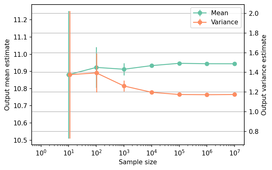
The tabulated results for each sample size is shown below.

Show code cell source Hide code cell source

from tabulate import tabulate

# --- Compile data row-wise
outputs = []
for (
    sample_size,
    mean_estimate,
    mean_estimate_error,
    var_estimate,
    var_estimate_error,
) in zip(
    sample_sizes,
    mean_estimates,
    mean_estimates_errors,
    var_estimates,
    var_estimates_errors,
):
    outputs += [
        [
            sample_size,
            mean_estimate,
            mean_estimate_error,
            var_estimate,
            var_estimate_error,
            "Monte-Carlo",
        ],
    ]

header_names = [
    "Sample size",
    "Mean",
    "Mean error",
    "Variance",
    "Variance error",
    "Remark",
]

tabulate(
    outputs,
    headers=header_names,
    floatfmt=(".1e", ".4e", ".4e", ".4e", ".4e", "s"),
    tablefmt="html",
    stralign="center",
    numalign="center",
)

Sample size	Mean	Mean error	Variance	Variance error	Remark
1.0e+01	1.0881e+01	3.7105e-01	1.3768e+00	6.4901e-01	Monte-Carlo
1.0e+02	1.0923e+01	1.1809e-01	1.3944e+00	1.9819e-01	Monte-Carlo
1.0e+03	1.0912e+01	3.5515e-02	1.2613e+00	5.6436e-02	Monte-Carlo
1.0e+04	1.0934e+01	1.0940e-02	1.1969e+00	1.6927e-02	Monte-Carlo
1.0e+05	1.0947e+01	3.4272e-03	1.1746e+00	5.2529e-03	Monte-Carlo
1.0e+06	1.0945e+01	1.0828e-03	1.1725e+00	1.6581e-03	Monte-Carlo
1.0e+07	1.0944e+01	3.4271e-04	1.1745e+00	5.2527e-04	Monte-Carlo

References

[IL15] (1,2)

Bertrand Iooss and Paul Lemaître. A review on global sensitivity analysis methods. In Uncertainty Management in Simulation-Optimization of Complex Systems, pages 101–122. Springer US, 2015. doi:10.1007/978-1-4899-7547-8_5.

[BDIP17]

Michaël Baudin, Anne Dutfoy, Bertrand Iooss, and Anne-Laure Popelin. OpenTURNS: an industrial software for uncertainty quantification in simulation. In Handbook of Uncertainty Quantification, pages 2001–2038. Springer International Publishing, 2017. doi:10.1007/978-3-319-12385-1_64.

[LIPG13]

M. Lamboni, B. Iooss, A.-L. Popelin, and F. Gamboa. Derivative-based global sensitivity measures: General links with Sobol' indices and numerical tests. Mathematics and Computers in Simulation, 87:45–54, 2013. doi:10.1016/j.matcom.2013.02.002.