Two-dimensional Polynomial Function from Lim et al. (2002)#
import numpy as np
import matplotlib.pyplot as plt
import uqtestfuns as uqtf
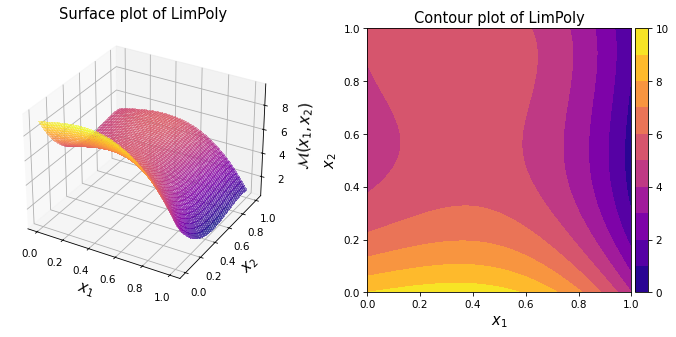
The polynomial test function from Lim et al. (2002) (or LimPoly for short)
is a two-dimensional scalar-valued function.
The function was used in [LSSW02] in the context of establishing the
connection between Gaussian process metamodel and polynomials.
Test function instance#
To create a default instance of the test function:
my_testfun = uqtf.LimPoly()
Check if it has been correctly instantiated:
print(my_testfun)
Function ID      : LimPoly
Input Dimension  : 2 (fixed)
Output Dimension : 1
Parameterized    : False
Description      : Two-dimensional polynomial function from Lim et al. (2002)
Applications     : metamodeling
Description#
The test function is defined as follows[1]:
where \(\boldsymbol{x} = \{ x_1, x_2 \}\) is the two-dimensional vector of input variables further defined below.
Note
The coefficients of the test function are chosen such that its global features are similar to its non-polynomial counterpart.
Probabilistic input#
The input consists of two uniformly distributed random variables as shown below.
Show code cell source
print(my_testfun.prob_input)
Function ID     : LimPoly
Input ID        : Lim2002
Input Dimension : 2
Description     : Input specification for the polynomial function from Lim
                  et al. (2002)
Marginals       :

 No.    Name    Distribution    Parameters    Description
-----  ------  --------------  ------------  -------------
  1      x1       uniform        [0. 1.]           -
  2      x2       uniform        [0. 1.]           -

Copulas         : Independence
Reference results#
This section provides several reference results of typical UQ analyses involving the test function.
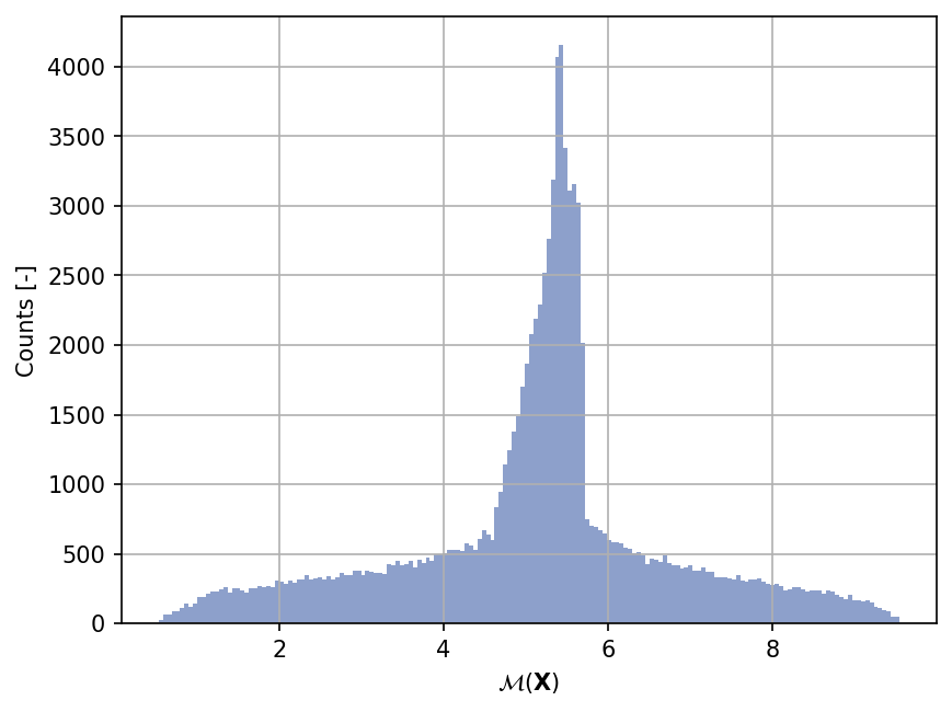
Sample histogram#
Shown below is the histogram of the output based on \(100'000\) random points:
Show code cell source
xx_test = my_testfun.prob_input.get_sample(100000)
yy_test = my_testfun(xx_test)

plt.hist(yy_test, bins="auto", color="#8da0cb");
plt.grid();
plt.ylabel("Counts [-]");
plt.xlabel("$\mathcal{M}(\mathbf{X})$");
plt.gcf().set_dpi(150);
References#
Yong B. Lim, Jerome Sacks, W. J. Studden, and William J. Welch. Design and analysis of computer experiments when the output is highly correlated over the input space. Canadian Journal of Statistics, 30(1):109–126, 2002. doi:10.2307/3315868.