Sobol’-Levitan Function

The Sobol’-Levitan function is an M-dimensional, scalar-valued function commonly used as a benchmark for sensitivity analysis. The function was introduced in [SobolL99] (as a six- and 20-dimensional functions) and revisited in, for example, [MDS12] (as a 20-dimensional function) and [SCJR22] (as a seven- and 15-dimensional functions).

import numpy as np
import matplotlib.pyplot as plt
import uqtestfuns as uqtf

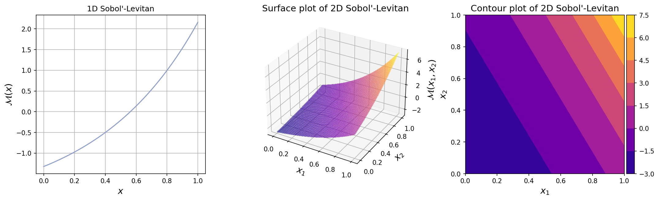
The plots for one-dimensional and two-dimensional Sobol’-Levitan function can be seen below.

Test function instance

To create a default instance of the Sobol’-Levitan function, type:

my_testfun = uqtf.SobolLevitan()

Check if it has been correctly instantiated:

print(my_testfun)

Function ID      : SobolLevitan
Input Dimension  : 2 (variable)
Output Dimension : 1
Parameterized    : True
Description      : Test function from Sobol' and Levitan (1999)
Applications     : sensitivity

By default, the input dimension is set to \(2\)[1]. To create an instance with another value of input dimension, pass an integer to the parameter input_dimension (the first parameter). For example, to create an instance of the Sobol’-Levitan function in six dimensions, type:

my_testfun = uqtf.SobolLevitan(input_dimension=6)

In the subsequent section, the function will be illustrated using six dimensions as it originally appeared in [SobolL99].

Description

The Sobol’-Levitan function is defined as follows[2]:

\[ \mathcal{M}(\boldsymbol{x}; \boldsymbol{b}, c_0) = \exp{\left[ \sum_{i = 1}^M b_i x_i \right]} - I_M(\boldsymbol{b}) + c_0, \]

where

\[ I_M (\boldsymbol{b}) = \prod_{i = 1}^M \frac{e^{b_i} - 1}{b_i}, \]

where \(\boldsymbol{x} = \{ x_1, \ldots, x_M \}\) is the \(M\)-dimensional vector of input variables further defined below, and \(\boldsymbol{b}\) and \(c_0\) are parameters of the function also further defined below.

Probabilistic input

The probabilistic input model for the Sobol’-Levitan function consists of \(M\) independent uniform random variables in \([0.0, 1.0]^M\).

For the selected input dimension, the input model is shown below.

Show code cell source Hide code cell source

print(my_testfun.prob_input)

Function ID     : SobolLevitan
Input ID        : Sobol1999
Input Dimension : 6
Description     : Probabilistic input model for the Sobol'-Levitan function
                  from Sobol' and Levitan (1999)
Marginals       :

 No.    Name    Distribution    Parameters    Description
-----  ------  --------------  ------------  -------------
  1      X1       uniform        [0. 1.]           -
  2      X2       uniform        [0. 1.]           -
  3      X3       uniform        [0. 1.]           -
  4      X4       uniform        [0. 1.]           -
  5      X5       uniform        [0. 1.]           -
  6      X6       uniform        [0. 1.]           -

Copulas         : Independence

Parameters

The parameters of the Sobol’-Levitan function consists of the coefficients \(\boldsymbol{b}\) and the constant term \(c_0\). The coefficients determine the importance of each input variables. The constant term, while influences the mean value of the function, does not alter the global sensitivity analysis.

The available parameters for the Sobol’-Levitan function are shown in the table below.

Table 9 Available parameters of the Sobol’-Levitan function

No.	\(\boldsymbol{b}\)	\(c_0\)	Keyword	Source	Remark
1.	\(b_1 = 1.5\) \(b_2 = \ldots = b_M = 0.9\)	\(0.0\)	Sobol1999-1 (default)	[SobolL99] (Example 6.1)	Originally, six dimensions
2.	\(b_1 = \ldots = b_{10} = 0.6\) \(b_{11} = \ldots = b_M = 0.4\)	\(0.0\)	Sobol1999-2	[SobolL99] (Example 6.2)	Originally, 20 dimensions
3.	\(\boldsymbol{b}_{1-20}\)[3] \(b_i = 0.0, i = 21, \ldots, M\)	\(0.0\)	Moon2012-1	[MDS12] (Table 7)	Originally, 20 dimensions

The default parameter is shown below.

Show code cell source Hide code cell source

print(my_testfun.parameters)

Function ID  : SobolLevitan
Parameter ID : Sobol1999-1
Description  : Parameter set for the M-dimensional function from Sobol'
               and Levitan (1999), 6D case

 No.    Keyword      Value      Type      Description
-----  ---------  -----------  -------  ----------------
  1       bb      (6,) array   ndarray  Coefficients 'b'
  2       c0      0.00000e+00   float    Constant term

Note

To create an instance of the Sobol’-Levitan function with different built-in parameter values, pass the corresponding keyword to the parameter parameters_id. For example, to use the parameters of Example 6.2 from [SobolL99], type:

my_testfun = uqtf.SobolLevitan(parameters_id="Sobol1999-2")

Attention

If the value of parameter \(b_i\) is zero then the value of \(\frac{e^{b_i} - 1}{b_i}\) that appears in the expression of \(I_M\) above is singular but in the limit is reduced to \(1.0\).

Reference results

This section provides several reference results of typical UQ analyses involving the test function.

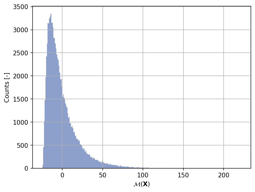
Sample histogram

Shown below is the histogram of the output based on \(100'000\) random points:

Show code cell source Hide code cell source

np.random.seed(42)
xx_test = my_testfun.prob_input.get_sample(100000)
yy_test = my_testfun(xx_test)

plt.hist(yy_test, bins="auto", color="#8da0cb");
plt.grid();
plt.ylabel("Counts [-]");
plt.xlabel("$\mathcal{M}(\mathbf{X})$");
plt.gcf().set_dpi(150);

Definite integration

The integral value of the function over the whole domain \([0, 1]^M\) is analytical:

\[ \int_{[0, 1]^M} \mathcal{M}(\boldsymbol{x}) \; d\boldsymbol{x} = c_0. \]

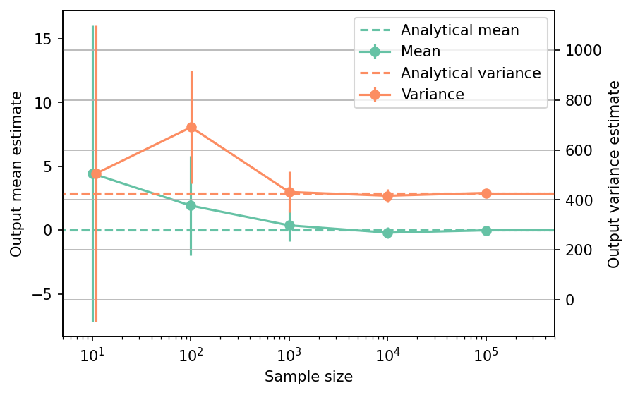
Moments

The mean and variance of the Sobol’-Levitan function can be computed analytically.

The mean[4] is given as follows:

\[ \mathbb{E}[Y] = c_0, \]

while the variance is given as follows:

\[ \mathbb{V}[Y] (\boldsymbol{b}) = H_M(\boldsymbol{b}) - I_Mˆ2(\boldsymbol{b}) \]

where \(I_M\) is given in the section above and

\[ H_M (\boldsymbol{b}) = \prod_{i = 1}^M \frac{e^{2 b_i} - 1}{2 b_i}. \]

Notice that the values of the mean and variance depend on the choice of the parameter values.

Shown below is the convergence of a direct Monte-Carlo estimation of the output mean and variance with increasing sample sizes compared with the analytical values. The error bars correspond to twice the standard deviation of the estimates obtained from \(50\) replications.

Show code cell source Hide code cell source

# --- Compute the mean and variance estimate
sample_sizes = np.array([1e1, 1e2, 1e3, 1e4, 1e5], dtype=int)
mean_estimates = np.empty((len(sample_sizes), 50))
var_estimates = np.empty((len(sample_sizes), 50))
my_testfun.prob_input.reset_rng(42)

for i, sample_size in enumerate(sample_sizes):
    for j in range(50):
        xx_test = my_testfun.prob_input.get_sample(sample_size)
        yy_test = my_testfun(xx_test)
        mean_estimates[i, j] = np.mean(yy_test)
        var_estimates[i, j] = np.var(yy_test)

mean_estimates_errors = np.std(mean_estimates, axis=1)
var_estimates_errors = np.std(var_estimates, axis=1)

# --- Compute analytical mean and variance
mean_analytical = my_testfun.parameters["c0"]
bb = my_testfun.parameters["bb"]
h_m = np.prod((np.exp(2 * bb) - 1) / 2 / bb)
i_m = np.prod((np.exp(bb) - 1) / bb)
var_analytical = h_m - i_m**2

# --- Plot the mean and variance estimates
fig, ax_1 = plt.subplots(figsize=(6,4))

ext_sample_sizes = np.insert(sample_sizes, 0, 1)
ext_sample_sizes = np.insert(ext_sample_sizes, -1, 5e6)

# --- Mean plot
ax_1.errorbar(
    sample_sizes,
    mean_estimates[:,0],
    yerr=2.0*mean_estimates_errors,
    marker="o",
    color="#66c2a5",
    label="Mean"
)
# Plot the analytical mean
ax_1.plot(
    ext_sample_sizes,
    np.repeat(mean_analytical, len(ext_sample_sizes)),
    linestyle="--",
    color="#66c2a5",
    label="Analytical mean",
)
ax_1.set_xlim([5, 5e5])
ax_1.set_xlabel("Sample size")
ax_1.set_ylabel("Output mean estimate")
ax_1.set_xscale("log");
ax_2 = ax_1.twinx()

# --- Variance plot
ax_2.errorbar(
    sample_sizes+1,
    var_estimates[:,0],
    yerr=2.0*var_estimates_errors,
    marker="o",
    color="#fc8d62",
    label="Variance",
)
# Plot the analytical variance
ax_2.plot(
    ext_sample_sizes,
    np.repeat(var_analytical, len(ext_sample_sizes)),
    linestyle="--",
    color="#fc8d62",
    label="Analytical variance",
)
ax_2.set_ylabel("Output variance estimate")

# Add the two plots together to have a common legend
ln_1, labels_1 = ax_1.get_legend_handles_labels()
ln_2, labels_2 = ax_2.get_legend_handles_labels()
ax_2.legend(ln_1 + ln_2, labels_1 + labels_2, loc=0)

plt.grid()
fig.set_dpi(150)

Sensitivity indices

The main-effect Sobol’ sensitivity indices of the Sobol’-Levitan function are given by the following formula:

\[ S_i = \frac{R_i - 1}{R_M - 1},\; i = 1, \ldots, M, \]

where

\[ R_M = \frac{H_M}{I_M^2};\;\; R_i = \frac{H_i}{I_i^2}, \]

and

\[ H_i = \frac{e^{2 b_i} - 1}{2 b_i};\;\; I_i = \frac{e^{b_i} - 1}{b_i}. \]

The total-effect Sobol’ sensitivity indices, on the other hand, are given by the following formula:

\[ ST_i = 1 - S_{\sim i}, \; i = 1, \ldots, M, \]

where

\[ S_{\sim i} = \frac{\left( R_M / R_i \right) - 1}{R_M - 1} \]

The formulas are general in the sense that assuming \(\boldsymbol{x}_a = (x_1, \ldots, x_a)\) and \(\boldsymbol{x}_b = (x_{a + 1}, \ldots, x_M)\) such that \(\boldsymbol{x} = (\boldsymbol{x}_a, \boldsymbol{x}_b)\), the sensitivity indices of the sets are:

\[ S_{a} = \frac{R_a - 1}{R_M - 1} \]

\[ S_{b} = \frac{(R_M / R_a) - 1}{R_M - 1} \]

\[ ST_{a} = 1 - S_{b}. \]

Some example values of the Sobol’ main- and total-effect sensitivity indices for the Sobol’-Levitan function with the three available parameter sets and the original dimension as appeared in the corresponding literature.

Sobol1999-1

Input	\(S_i\)	\(ST_i\)
\(X_1\)	\(2.86993e \times 10^{-1}\)	\(3.96179 \times 10^{-1}\)
\(X_2\)	\(1.05712e \times 10^{-1}\)	\(1.61558 \times 10^{-1}\)
\(X_3\)	\(1.05712e \times 10^{-1}\)	\(1.61558 \times 10^{-1}\)
\(X_4\)	\(1.05712e \times 10^{-1}\)	\(1.61558 \times 10^{-1}\)
\(X_5\)	\(1.05712e \times 10^{-1}\)	\(1.61558 \times 10^{-1}\)
\(X_6\)	\(1.05712e \times 10^{-1}\)	\(1.61558 \times 10^{-1}\)

Sobol1999-2

Input	\(S_i\)	\(ST_i\)
\(X_1\)	\(5.61551 \times 10^{-2}\)	\(8.34869 \times 10^{-2}\)
\(X_2\)	\(5.61551 \times 10^{-2}\)	\(8.34869 \times 10^{-2}\)
\(X_3\)	\(5.61551 \times 10^{-2}\)	\(8.34869 \times 10^{-2}\)
\(X_4\)	\(5.61551 \times 10^{-2}\)	\(8.34869 \times 10^{-2}\)
\(X_5\)	\(5.61551 \times 10^{-2}\)	\(8.34869 \times 10^{-2}\)
\(X_6\)	\(5.61551 \times 10^{-2}\)	\(8.34869 \times 10^{-2}\)
\(X_7\)	\(5.61551 \times 10^{-2}\)	\(8.34869 \times 10^{-2}\)
\(X_8\)	\(5.61551 \times 10^{-2}\)	\(8.34869 \times 10^{-2}\)
\(X_9\)	\(5.61551 \times 10^{-2}\)	\(8.34869 \times 10^{-2}\)
\(X_{10}\)	\(5.61551 \times 10^{-2}\)	\(8.34869 \times 10^{-2}\)
\(X_{11}\)	\(2.50405 \times 10^{-2}\)	\(3.78353 \times 10^{-2}\)
\(X_{12}\)	\(2.50405 \times 10^{-2}\)	\(3.78353 \times 10^{-2}\)
\(X_{13}\)	\(2.50405 \times 10^{-2}\)	\(3.78353 \times 10^{-2}\)
\(X_{14}\)	\(2.50405 \times 10^{-2}\)	\(3.78353 \times 10^{-2}\)
\(X_{15}\)	\(2.50405 \times 10^{-2}\)	\(3.78353 \times 10^{-2}\)
\(X_{16}\)	\(2.50405 \times 10^{-2}\)	\(3.78353 \times 10^{-2}\)
\(X_{17}\)	\(2.50405 \times 10^{-2}\)	\(3.78353 \times 10^{-2}\)
\(X_{18}\)	\(2.50405 \times 10^{-2}\)	\(3.78353 \times 10^{-2}\)
\(X_{19}\)	\(2.50405 \times 10^{-2}\)	\(3.78353 \times 10^{-2}\)
\(X_{20}\)	\(2.50405 \times 10^{-2}\)	\(3.78353 \times 10^{-2}\)

Moon2012-1

Input	\(S_i\)	\(ST_i\)
\(X_1\)	\(5.49487 \times 10^{-2}\)	\(2.80254 \times 10^{-1}\)
\(X_2\)	\(5.23891 \times 10^{-2}\)	\(2.70200 \times 10^{-1}\)
\(X_3\)	\(4.98801 \times 10^{-2}\)	\(2.60124 \times 10^{-1}\)
\(X_4\)	\(4.74227 \times 10^{-2}\)	\(2.50034 \times 10^{-1}\)
\(X_5\)	\(4.50178 \times 10^{-2}\)	\(2.39943 \times 10^{-1}\)
\(X_6\)	\(4.26663 \times 10^{-2}\)	\(2.29860 \times 10^{-1}\)
\(X_7\)	\(4.03691 \times 10^{-2}\)	\(2.19798 \times 10^{-1}\)
\(X_8\)	\(3.81272 \times 10^{-2}\)	\(2.09769 \times 10^{-1}\)
\(X_9\)	\(2.60713 \times 10^{-3}\)	\(1.72041 \times 10^{-2}\)
\(X_{10}\)	\(1.38278 \times 10^{-3}\)	\(9.18792 \times 10^{-3}\)
\(X_{11}\)	\(6.87641 \times 10^{-4}\)	\(4.58707 \times 10^{-3}\)
\(X_{12}\)	\(3.16411 \times 10^{-4}\)	\(2.11515 \times 10^{-3}\)
\(X_{13}\)	\(1.32275 \times 10^{-4}\)	\(8.85162 \times 10^{-4}\)
\(X_{14}\)	\(4.86979 \times 10^{-5}\)	\(3.26033 \times 10^{-4}\)
\(X_{15}\)	\(1.52609 \times 10^{-5}\)	\(1.02191 \times 10^{-4}\)
\(X_{16}\)	\(3.79169 \times 10^{-6}\)	\(2.53919 \times 10^{-5}\)
\(X_{17}\)	\(6.76395 \times 10^{-7}\)	\(4.52971 \times 10^{-6}\)
\(X_{18}\)	\(6.45092 \times 10^{-8}\)	\(4.32009 \times 10^{-7}\)
\(X_{19}\)	\(2.34038 \times 10^{-9}\)	\(1.56732 \times 10^{-8}\)
\(X_{20}\)	\(0.00000\)	\(0.00000\)

References

[SCJR22]

Xifu Sun, Barry Croke, Anthony Jakeman, and Stephen Roberts. Benchmarking Active Subspace methods of global sensitivity analysis against variance-based Sobol’ and Morris methods with established test functions. Environmental Modelling & Software, 149:105310, 2022. doi:10.1016/j.envsoft.2022.105310.

[SobolL99] (1,2,3,4,5,6)

Ilya M. Sobol' and Yu L. Levitan. On the use of variance reducing multipliers in Monte Carlo computations of a global sensitivity index. Computer Physics Communications, 117(1):52–61, 1999. doi:10.1016/S0010-4655(98)00156-8.

[MDS12] (1,2)

Hyejung Moon, Angela M. Dean, and Thomas J. Santner. Two-stage sensitivity-based group screening in computer experiments. Technometrics, 54(4):376–387, 2012. doi:10.1080/00401706.2012.725994.

---

[1]

This default dimension applies to all variable dimension test functions. It will be used if the input_dimension argument is not given.

[2]

see Section 4, pp. 55-56 [SobolL99].

[3]

\(\boldsymbol{b}_{1 - 5} = \left(2.0000, 1.9500, 1.9000, 1.8500, 1.8000 \right)\), \(\boldsymbol{b}_{6 - 10} = \left( 1.7500, 1.7000, 1.6500, 0.4228, 0.3077 \right)\), \(\boldsymbol{b}_{11 - 15} = \left( 0.2169, 0.1471, 0.0951, 0.0577, 0.0323 \right)\), and \(\boldsymbol{b}_{16 - 20} = \left( 0.0161, 0.0068, 0.0021, 0.0004, 0.0000 \right)\).

[4]

The expected value is the same as the integral over the domain because the input is uniform in a unit hypercube.