McLain S1 Function#
import numpy as np
import matplotlib.pyplot as plt
import uqtestfuns as uqtf
The McLain S1 function is a two-dimensional scalar-valued function. The function was introduced in [McL74] as a test function for procedures to construct contours from a given set of points.
Note
The McLain’s test functions are a set of five two-dimensional functions that mathematically defines surfaces. The functions are:
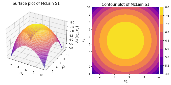
As shown in the plots above, the resulting surface is a part of a sphere. The center of the sphere is at \((5.5, 5.5)\) and the maximum height is \(8.0\).
Note
The McLain S1 function appeared in a modified form in the report of Franke [Fra79] (specifically the (6th) Franke function).
In fact, four of the Franke’s test functions (2, 4, 5, and 6) are slight modifications of the McLain’s, including the translation of the input domain from \([1.0, 10.0]^2\) to \([0.0, 1.0]^2\).
Test function instance#
To create a default instance of the McLain S1 function:
my_testfun = uqtf.McLainS1()
Check if it has been correctly instantiated:
print(my_testfun)
Function ID      : McLainS1
Input Dimension  : 2 (fixed)
Output Dimension : 1
Parameterized    : False
Description      : McLain S1 function from McLain (1974)
Applications     : metamodeling
Description#
The McLain S1 function is defined as follows:
where \(\boldsymbol{x} = \{ x_1, x_2 \}\) is the two-dimensional vector of input variables further defined below.
Probabilistic input#
Based on [McL74], the probabilistic input model for the function consists of two independent random variables as shown below.
Show code cell source
print(my_testfun.prob_input)
Function ID     : McLain
Input ID        : McLain1974
Input Dimension : 2
Description     : Input specification for the McLain's test functions from
                  McLain (1974).
Marginals       :

 No.    Name    Distribution    Parameters    Description
-----  ------  --------------  ------------  -------------
  1      X1       uniform       [ 1. 10.]          -
  2      X2       uniform       [ 1. 10.]          -

Copulas         : Independence
Reference results#
This section provides several reference results of typical UQ analyses involving the test function.
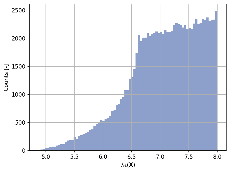
Sample histogram#
Shown below is the histogram of the output based on \(100'000\) random points:
Show code cell source
xx_test = my_testfun.prob_input.get_sample(100000)
yy_test = my_testfun(xx_test)

plt.hist(yy_test, bins="auto", color="#8da0cb");
plt.grid();
plt.ylabel("Counts [-]");
plt.xlabel("$\mathcal{M}(\mathbf{X})$");
plt.gcf().set_dpi(150);
References#
Richard Franke. A critical comparison of some methods for interpolation of scattered data. techreport NPS53-79-003, Naval Postgraduate School, Monterey, Canada, 1979. URL: https://core.ac.uk/reader/36727660.
D. H. McLain. Drawing contours from arbitrary data points. The Computer Journal, 17(4):318–324, 1974. doi:10.1093/comjnl/17.4.318.