McLain S4 Function#
import numpy as np
import matplotlib.pyplot as plt
import uqtestfuns as uqtf
The McLain S4 function is a two-dimensional scalar-valued function. The function was introduced in [McL74] as a test function for procedures to construct contours from a given set of points.
Note
The McLain’s test functions are a set of five two-dimensional functions that mathematically defines surfaces. The functions are:
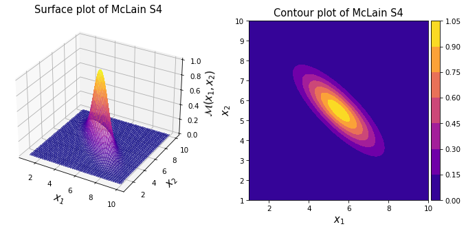
As shown in the plots above, the resulting surface consists of a long narrow hill running diagonally from \((0.0, 10.0)\) to \((10.0, 0.0)\). The maximum height is \(1.0\) at \((5.5, 5.5)\).
Test function instance#
To create a default instance of the McLain S4 function:
my_testfun = uqtf.McLainS4()
Check if it has been correctly instantiated:
print(my_testfun)
Function ID      : McLainS4
Input Dimension  : 2 (fixed)
Output Dimension : 1
Parameterized    : False
Description      : McLain S4 function from McLain (1974)
Applications     : metamodeling
Description#
The McLain S4 function is defined as follows:
where \(\boldsymbol{x} = \{ x_1, x_2 \}\) is the two-dimensional vector of input variables further defined below.
Probabilistic input#
Based on [McL74], the probabilistic input model for the function consists of two independent random variables as shown below.
Show code cell source
print(my_testfun.prob_input)
Function ID     : McLain
Input ID        : McLain1974
Input Dimension : 2
Description     : Input specification for the McLain's test functions from
                  McLain (1974).
Marginals       :

 No.    Name    Distribution    Parameters    Description
-----  ------  --------------  ------------  -------------
  1      X1       uniform       [ 1. 10.]          -
  2      X2       uniform       [ 1. 10.]          -

Copulas         : Independence
Reference results#
This section provides several reference results of typical UQ analyses involving the test function.
Sample histogram#
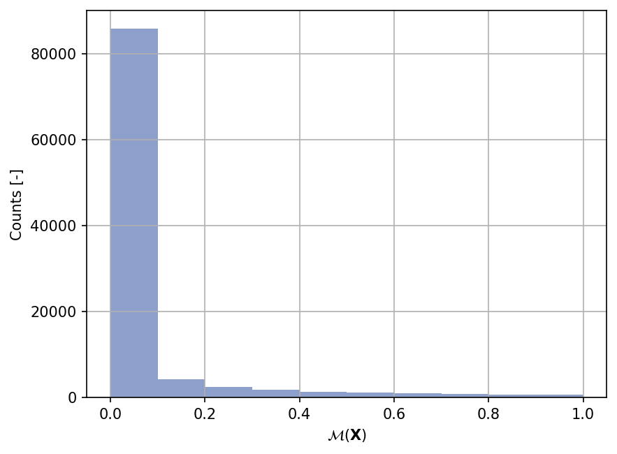
Shown below is the histogram of the output based on \(100'000\) random points:
Show code cell source
xx_test = my_testfun.prob_input.get_sample(100000)
yy_test = my_testfun(xx_test)

plt.hist(yy_test, color="#8da0cb");
plt.grid();
plt.ylabel("Counts [-]");
plt.xlabel("$\mathcal{M}(\mathbf{X})$");
plt.gcf().set_dpi(150);
References#
D. H. McLain. Drawing contours from arbitrary data points. The Computer Journal, 17(4):318–324, 1974. doi:10.1093/comjnl/17.4.318.