Sine Function from Holsclaw et al. (2013)#
import numpy as np
import matplotlib.pyplot as plt
import uqtestfuns as uqtf
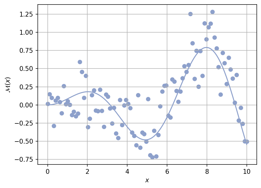
The function is a simple one-dimensional, scalar-valued test function. It was featured in [HSL+13] as an example for computing the derivative of a curve using Gaussian process.
A plot of the function is shown below..
Note
In the original paper, the function was evaluated at 100 equispaced points in \([0, 10.0]\) with added i.i.d noise from \(\mathcal{N} \sim (0, 0.3)\); these points are shown in the above plot.
Test function instance#
To create a default instance of the test function:
my_testfun = uqtf.HolsclawSine()
Check if it has been correctly instantiated:
print(my_testfun)
Function ID      : HolsclawSine
Input Dimension  : 1 (fixed)
Output Dimension : 1
Parameterized    : False
Description      : Sine function from Holsclaw et al. (2013)
Applications     : metamodeling
Description#
The test function is analytically defined as follows[1]:
where \(x\) is further defined below.
Probabilistic input#
The probabilistic input model for the test function is shown below.
Show code cell source
print(my_testfun.prob_input)
Function ID     : HolsclawSine
Input ID        : Holsclaw2013
Input Dimension : 1
Description     : Input model for the sine function from Holsclaw et al.
                  (2013)
Marginals       :

 No.    Name    Distribution    Parameters    Description
-----  ------  --------------  ------------  -------------
  1      x        uniform       [ 0. 10.]          -
Reference results#
This section provides several reference results of typical UQ analyses involving the test function.
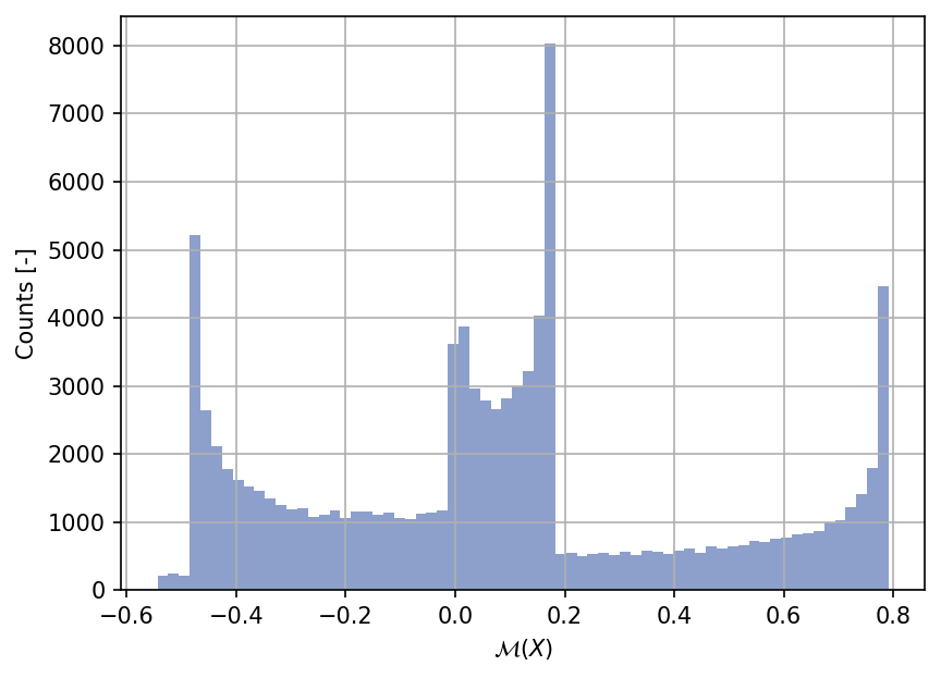
Sample histogram#
Shown below is the histogram of the output based on \(100'000\) random points:
Show code cell source
my_testfun.prob_input.reset_rng(42)
xx_test = my_testfun.prob_input.get_sample(100000)
yy_test = my_testfun(xx_test)

plt.hist(yy_test, bins="auto", color="#8da0cb");
plt.grid();
plt.ylabel("Counts [-]");
plt.xlabel("$\mathcal{M}(X)$");
plt.gcf().tight_layout(pad=3.0)
plt.gcf().set_dpi(150);
References#
Tracy Holsclaw, Bruno Sansó, Herbert K. H. Lee, Katrin Heitmann, Salman Habib, David Higdon, and Ujjaini Alam. Gaussian process modeling of derivative curves. Technometrics, 55(1):57–67, 2013. doi:10.1080/00401706.2012.723918.