(2nd) Franke Function

import numpy as np
import matplotlib.pyplot as plt
import uqtestfuns as uqtf

The (2nd) Franke function is a two-dimensional scalar-valued function. The function was introduced in [Fra79] in the context of interpolation problem.

Note

The Franke’s original report [Fra79] contains in total six two-dimensional test functions:

• (1st) Franke function: Two Gaussian peaks and a Gaussian dip on a surface slopping down the upper right boundary

• (2nd) Franke function: Two nearly flat regions joined by a sharp rise running diagonally (this function)

• (3rd) Franke function: A saddle shaped surface

• (4th) Franke function: A Gaussian hill that slopes off in a gentle fashion

• (5th) Franke function: A steep Gaussian hill that approaches zero at the boundaries

• (6th) Franke function: A part of a sphere

The term “Franke function” typically only refers to the (1st) Franke function.

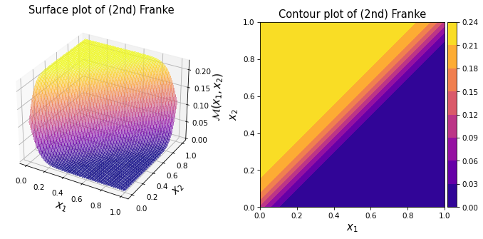
As shown in the plots above, the function features two nearly flat regions of height \(0.0\) and (approximately) \(\frac{2}{9}\). The two regions are joined by a sharp rise that runs diagonally from \((0.0, 0.0)\) to \((1.0, 1.0)\).

Note

The (2nd) Franke function is a modified form of the McLain S5 function [McL74].

Specifically, the domain of the function is translated from \([1.0, 10.0]^2\) to \([0.0, 1.0]^2\) with some additional slight modifications to “enhance the visual aspects” of the resulting surfaces.

Test function instance

To create a default instance of the (2nd) Franke function:

my_testfun = uqtf.Franke2()

Check if it has been correctly instantiated:

print(my_testfun)

Function ID      : Franke2
Input Dimension  : 2 (fixed)
Output Dimension : 1
Parameterized    : False
Description      : (2nd) Franke function from Franke (1979)
Applications     : metamodeling

Description

The (2nd) Franke function is defined as follows:

\[ \mathcal{M}(\boldsymbol{x}) = \frac{1}{9} \left( \tanh{(9 (x_2 - x_1))} + 1 \right) \]

where \(\boldsymbol{x} = \{ x_1, x_2 \}\) is the two-dimensional vector of input variables further defined below.

Probabilistic input

Based on [Fra79], the probabilistic input model for the function consists of two independent random variables as shown below.

Show code cell source Hide code cell source

print(my_testfun.prob_input)

Function ID     : Franke
Input ID        : Franke1979
Input Dimension : 2
Description     : Input specification for the test functions from Franke
                  (1979).
Marginals       :

 No.    Name    Distribution    Parameters    Description
-----  ------  --------------  ------------  -------------
  1      X1       uniform        [0. 1.]           -
  2      X2       uniform        [0. 1.]           -

Copulas         : Independence

Reference results

This section provides several reference results of typical UQ analyses involving the test function.

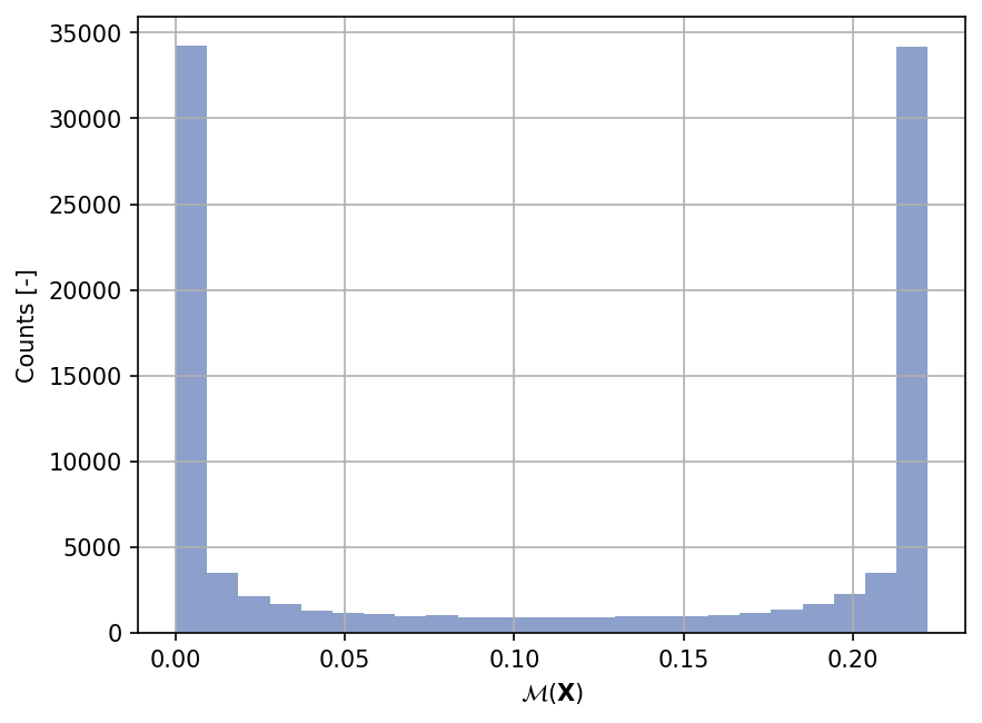
Sample histogram

Shown below is the histogram of the output based on \(100'000\) random points:

Show code cell source Hide code cell source

xx_test = my_testfun.prob_input.get_sample(100000)
yy_test = my_testfun(xx_test)

plt.hist(yy_test, bins="auto", color="#8da0cb");
plt.grid();
plt.ylabel("Counts [-]");
plt.xlabel("$\mathcal{M}(\mathbf{X})$");
plt.gcf().set_dpi(150);

References

[Fra79] (1,2,3)

Richard Franke. A critical comparison of some methods for interpolation of scattered data. techreport NPS53-79-003, Naval Postgraduate School, Monterey, Canada, 1979. URL: https://core.ac.uk/reader/36727660.

[McL74]

D. H. McLain. Drawing contours from arbitrary data points. The Computer Journal, 17(4):318–324, 1974. doi:10.1093/comjnl/17.4.318.