Wing Weight Function#
import numpy as np
import matplotlib.pyplot as plt
import uqtestfuns as uqtf
The Wing Weight test function [FSK08] is a 10-dimensional scalar-valued function. The function has been used as a test function in the context of metamodeling [ZZP+20] and optimization [FSK08].
Test function instance#
To create a default instance of the wing weight test function:
my_testfun = uqtf.WingWeight()
Check if it has been correctly instantiated:
print(my_testfun)
Function ID      : WingWeight
Input Dimension  : 10 (fixed)
Output Dimension : 1
Parameterized    : False
Description      : Wing weight model from Forrester et al. (2008)
Applications     : metamodeling, sensitivity
Description#
The weight of a light aircraft wing is computed using the following analytical expression:
where \(\boldsymbol{x} = \{ S_w, W_{fw}, A, \Lambda, q, \lambda, t_c, N_z, W_{dg}, W_p\}\) is the vector of input variables defined below.
Probabilistic input#
Based on [FSK08], the probabilistic input model for the Wing Weight function consists of eight independent uniform random variables with ranges shown in the table below.
Show code cell source
print(my_testfun.prob_input)
Function ID     : WingWeight
Input ID        : Forrester2008
Input Dimension : 10
Description     : Probabilistic input model for the Wing Weight model from
                  Forrester et al. (2008).
Marginals       :

 No.    Name    Distribution    Parameters                 Description
-----  ------  --------------  -------------  -------------------------------------
  1      Sw       uniform       [150. 200.]             wing area [ft^2]
  2     Wfw       uniform       [220. 300.]      weight of fuel in the wing [lb]
  3      A        uniform        [ 6. 10.]              aspect ratio [-]
  4    Lambda     uniform       [-10.  10.]       quarter-chord sweep [degrees]
  5      q        uniform        [16. 45.]    dynamic pressure at cruise [lb/ft^2]
  6    lambda     uniform        [0.5 1. ]               taper ratio [-]
  7      tc       uniform       [0.08 0.18]   aerofoil thickness to chord ratio [-]
  8      Nz       uniform        [2.5 6. ]          ultimate load factor [-]
  9     Wdg       uniform       [1700 2500]      flight design gross weight [lb]
 10      Wp       uniform      [0.025 0.08 ]         paint weight [lb/ft^2]

Copulas         : Independence
Reference Results#
This section provides several reference results of typical UQ analyses involving the test function.
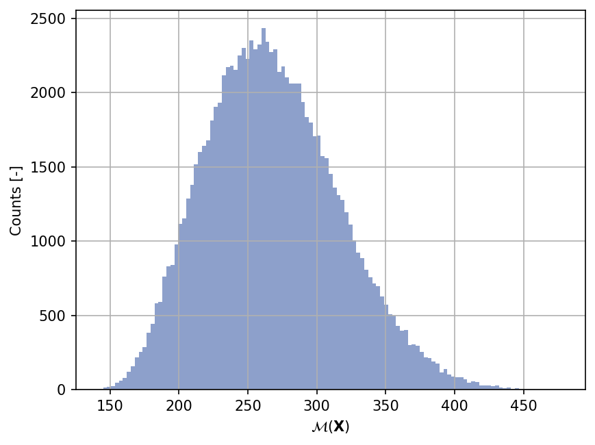
Sample histogram#
Shown below is the histogram of the output based on \(100'000\) random points:
Show code cell source
np.random.seed(42)
xx_test = my_testfun.prob_input.get_sample(100000)
yy_test = my_testfun(xx_test)

plt.hist(yy_test, bins="auto", color="#8da0cb");
plt.grid();
plt.ylabel("Counts [-]");
plt.xlabel("$\mathcal{M}(\mathbf{X})$");
plt.gcf().set_dpi(150);
Moments estimation#
Shown below is the convergence of a direct Monte-Carlo estimation of the output mean and variance with increasing sample sizes.
Show code cell source
# --- Compute the mean and variance estimate
np.random.seed(42)
sample_sizes = np.array([1e1, 1e2, 1e3, 1e4, 1e5, 1e6, 1e7], dtype=int)
mean_estimates = np.empty(len(sample_sizes))
var_estimates = np.empty(len(sample_sizes))

for i, sample_size in enumerate(sample_sizes):
    xx_test = my_testfun.prob_input.get_sample(sample_size)
    yy_test = my_testfun(xx_test)
    mean_estimates[i] = np.mean(yy_test)
    var_estimates[i] = np.var(yy_test)

# --- Compute the error associated with the estimates
mean_estimates_errors = np.sqrt(var_estimates) / np.sqrt(np.array(sample_sizes))
var_estimates_errors = var_estimates * np.sqrt(2 / (np.array(sample_sizes) - 1))

# --- Do the plot
fig, ax_1 = plt.subplots(figsize=(6,4))

ax_1.errorbar(
    sample_sizes,
    mean_estimates,
    yerr=mean_estimates_errors,
    marker="o",
    color="#66c2a5",
    label="Mean",
)
ax_1.set_xlabel("Sample size")
ax_1.set_ylabel("Output mean estimate")
ax_1.set_xscale("log");
ax_2 = ax_1.twinx()
ax_2.errorbar(
    sample_sizes + 1,
    var_estimates,
    yerr=var_estimates_errors,
    marker="o",
    color="#fc8d62",
    label="Variance",
)
ax_2.set_ylabel("Output variance estimate")

# Add the two plots together to have a common legend
ln_1, labels_1 = ax_1.get_legend_handles_labels()
ln_2, labels_2 = ax_2.get_legend_handles_labels()
ax_2.legend(ln_1 + ln_2, labels_1 + labels_2, loc=0)

plt.grid()
fig.set_dpi(150)
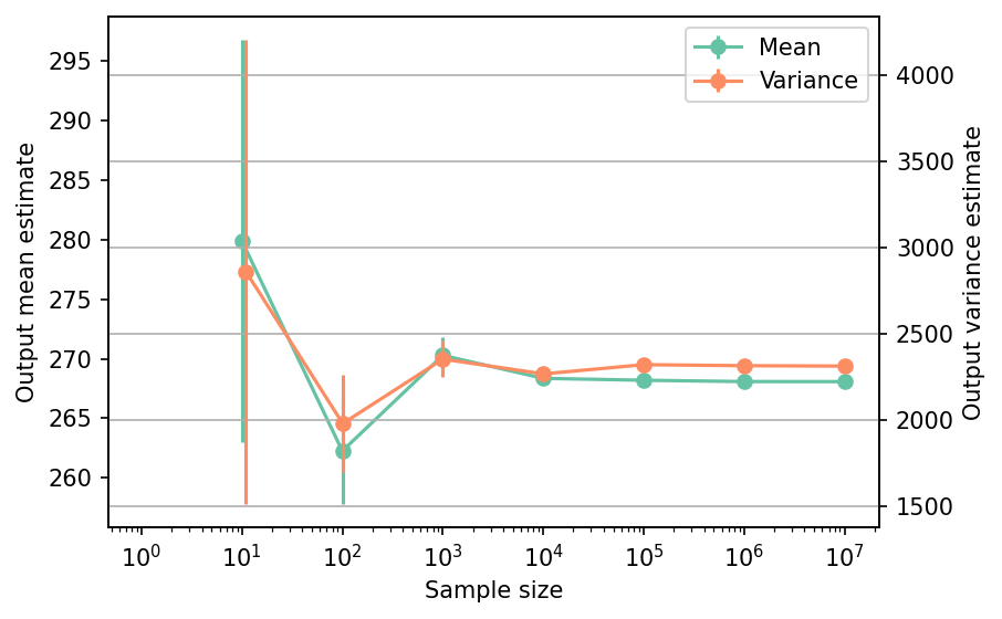
The tabulated results for each sample size is shown below.
Show code cell source
from tabulate import tabulate

# --- Compile data row-wise
outputs = []
for (
    sample_size,
    mean_estimate,
    mean_estimate_error,
    var_estimate,
    var_estimate_error,
) in zip(
    sample_sizes,
    mean_estimates,
    mean_estimates_errors,
    var_estimates,
    var_estimates_errors,
):
    outputs += [
        [
            sample_size,
            mean_estimate,
            mean_estimate_error,
            var_estimate,
            var_estimate_error,
            "Monte-Carlo",
        ],
    ]

header_names = [
    "Sample size",
    "Mean",
    "Mean error",
    "Variance",
    "Variance error",
    "Remark",
]

tabulate(
    outputs,
    headers=header_names,
    floatfmt=(".1e", ".4e", ".4e", ".4e", ".4e", "s"),
    tablefmt="html",
    stralign="center",
    numalign="center",
)
| Sample size | Mean | Mean error | Variance | Variance error | Remark |
|---|---|---|---|---|---|
| 1.0e+01 | 2.7989e+02 | 1.6908e+01 | 2.8587e+03 | 1.3476e+03 | Monte-Carlo |
| 1.0e+02 | 2.6225e+02 | 4.4473e+00 | 1.9778e+03 | 2.8112e+02 | Monte-Carlo |
| 1.0e+03 | 2.7028e+02 | 1.5336e+00 | 2.3519e+03 | 1.0523e+02 | Monte-Carlo |
| 1.0e+04 | 2.6835e+02 | 4.7601e-01 | 2.2659e+03 | 3.2046e+01 | Monte-Carlo |
| 1.0e+05 | 2.6819e+02 | 1.5230e-01 | 2.3195e+03 | 1.0373e+01 | Monte-Carlo |
| 1.0e+06 | 2.6808e+02 | 4.8100e-02 | 2.3136e+03 | 3.2719e+00 | Monte-Carlo |
| 1.0e+07 | 2.6807e+02 | 1.5203e-02 | 2.3113e+03 | 1.0336e+00 | Monte-Carlo |
References#
Alexander I. J. Forrester, András Sóbester, and Andy J. Keane. Engineering Design via Surrogate Modelling: A Practical Guide. Wiley, 1 edition, 2008. ISBN 978-0-470-06068-1 978-0-470-77080-1. doi:10.1002/9780470770801.
Lavi R. Zuhal, Kemas Zakaria, Pramudita S. Palar, Koji Shimoyama, and Rhea P. Liem. Gradient-enhanced universal Kriging with polynomial chaos as trend function. In AIAA Scitech 2020 Forum. Orlando, Florida, 2020. American Institute of Aeronautics and Astronautics. doi:10.2514/6.2020-1865.