Exponential Function from Dette and Pepelyshev (2010)#
import numpy as np
import matplotlib.pyplot as plt
import uqtestfuns as uqtf
The function is a three-dimensional, scalar-valued function that exhibits asymptotic behavior where the function value approaches zero near the origin and increases toward a value as the input moves farther away from the origin in any direction.
The function appeared in [DP10] as a test function for comparing different experimental designs in the construction of metamodels.
Test function instance#
To create a default instance of the test function:
my_testfun = uqtf.DetteExp()
Check if it has been correctly instantiated:
print(my_testfun)
Function ID      : DetteExp
Input Dimension  : 3 (fixed)
Output Dimension : 1
Parameterized    : False
Description      : Exponential function from Dette and Pepelyshev (2010)
Applications     : metamodeling
Description#
The test function is defined as[1]:
where \(\boldsymbol{x} = \left( x_1, x_2, x_3 \right)\) is the three-dimensional vector of input variables further defined below.
Probabilistic input#
The probabilistic input model for the test function is shown below.
Show code cell source
print(my_testfun.prob_input)
Function ID     : DetteExp
Input ID        : Dette2010
Input Dimension : 3
Description     : Input specification for the exponential test function
                  from Dette and Pepelyshev (2010)
Marginals       :

 No.    Name    Distribution    Parameters    Description
-----  ------  --------------  ------------  -------------
  1     x_1       uniform         [0 1]            -
  2     x_2       uniform         [0 1]            -
  3     x_3       uniform         [0 1]            -

Copulas         : Independence
Reference results#
This section provides several reference results of typical UQ analyses involving the test function.
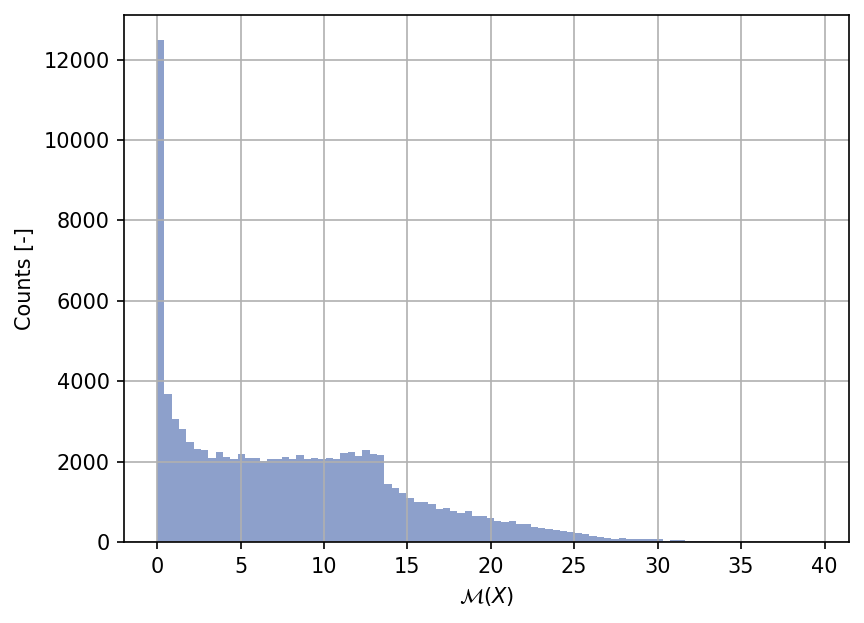
Sample histogram#
Shown below is the histogram of the output based on \(100'000\) random points:
Show code cell source
my_testfun.prob_input.reset_rng(42)
xx_test = my_testfun.prob_input.get_sample(100000)
yy_test = my_testfun(xx_test)

plt.hist(yy_test, bins="auto", color="#8da0cb");
plt.grid();
plt.ylabel("Counts [-]");
plt.xlabel("$\mathcal{M}(X)$");
plt.gcf().tight_layout(pad=3.0)
plt.gcf().set_dpi(150);
References#
Holger Dette and Andrey Pepelyshev. Generalized latin hypercube design for computer experiments. Technometrics, 52(4):421–429, 2010. doi:10.1198/tech.2010.09157.