Six-dimensional (6D) Friedman Function#
The 6D Friedman function (or Friedman6D function for short) is
a six-dimensional (including one dummy variable) scalar-valued function.
The function features a combination of non-linearity and variable interaction.
It was originally used in [FGS83] as a test function for testing a spline approximation method. In [SCJR22] and [HPS21] (albeit in a modified form) the function was employed as a test function in the context of sensitivity analysis.
Note
The function was later extended to ten dimension by incorporating four additional dummy variables (for a total of five) in [Fri91]; the function is also available in UQTestFuns.
import numpy as np
import matplotlib.pyplot as plt
import uqtestfuns as uqtf
Test function instance#
To create a default instance of the test function:
my_testfun = uqtf.Friedman6D()
Check if it has been correctly instantiated:
print(my_testfun)
Function ID      : Friedman6D
Input Dimension  : 6 (fixed)
Output Dimension : 1
Parameterized    : False
Description      : Six-dimensional function from Friedman et al. (1983)
Applications     : metamodeling, sensitivity
Description#
The test function is analytically defined as follows:
where \(x\) is defined below. Notice that the sixth input variable is inert.
Probabilistic input#
Based on [FGS83], the probabilistic input model for the function consists of two independent random variables as shown below.
Show code cell source
print(my_testfun.prob_input)
Function ID     : Friedman6D
Input ID        : Friedman1983
Input Dimension : 6
Description     : Input specification for the 6D test function from
                  Friedman et al. (1983)
Marginals       :

 No.    Name    Distribution    Parameters    Description
-----  ------  --------------  ------------  -------------
  1     x_1       uniform         [0 1]            -
  2     x_2       uniform         [0 1]            -
  3     x_3       uniform         [0 1]            -
  4     x_4       uniform         [0 1]            -
  5     x_5       uniform         [0 1]            -
  6     x_6       uniform         [0 1]            -

Copulas         : Independence
Reference results#
This section provides several reference results of typical UQ analyses involving the test function.
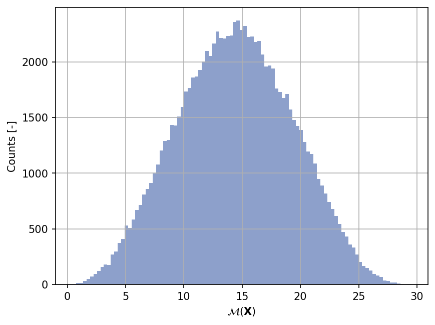
Sample histogram#
Shown below is the histogram of the output based on \(100'000\) random points:
Show code cell source
xx_test = my_testfun.prob_input.get_sample(100000)
yy_test = my_testfun(xx_test)

plt.hist(yy_test, bins="auto", color="#8da0cb");
plt.grid();
plt.ylabel("Counts [-]");
plt.xlabel("$\mathcal{M}(\mathbf{X})$");
plt.gcf().set_dpi(150);
References#
J. H. Friedman. Multivariate adaptive regression splines. The Annals of Statistics, 1991. doi:10.1214/aos/1176347963.
J. H. Friedman, E. Grosse, and W. Stuetzle. Multidimensional additive spline approximation. SIAM Journal on Scientific and Statistical Computing, 1983.
Akira Horiguchi, Matthew T. Pratola, and Thomas J. Santner. Assessing variable activity for Bayesian regression trees. Reliability Engineering & System Safety, 207:107391, March 2021. doi:10.1016/j.ress.2020.107391.
Xifu Sun, Barry Croke, Anthony Jakeman, and Stephen Roberts. Benchmarking Active Subspace methods of global sensitivity analysis against variance-based Sobol’ and Morris methods with established test functions. Environmental Modelling & Software, 149:105310, 2022. doi:10.1016/j.envsoft.2022.105310.