Test Function from Morris et al. (2006)#
The test function from Morris et al. (2006) [MMM06]
(or Morris2006 for short) is an \(M\)-dimensional scalar-valued function used
in the context of sensitivity analysis
[HPS21, SCJR22, MMM06].
The function features a parameter that controls the number of important input variables; the remaining variables, if any, are inert. Furthermore, the Sobol’ main-effect and total-effect sensitivity indices are the same for each input variable.
import numpy as np
import matplotlib.pyplot as plt
import uqtestfuns as uqtf
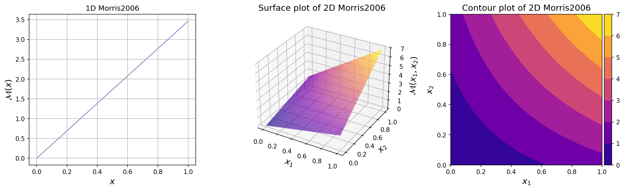
The plots for one-dimensional and two-dimensional Morris2006 function
can be seen below.
Test function instance#
To create a default instance of the function, type:
my_testfun = uqtf.Morris2006()
Check if it has been correctly instantiated:
print(my_testfun)
Function ID      : Morris2006
Input Dimension  : 2 (variable)
Output Dimension : 1
Parameterized    : True
Description      : Test function from Morris et al. (2006)
Applications     : sensitivity
By default, the input dimension is set to \(2\)[1].
To create an instance with another value of input dimension,
pass an integer to the parameter input_dimension (the first parameter).
For example, to create an instance of the function in 30 dimensions,
type:
my_testfun = uqtf.Morris2006(input_dimension=30)
In the subsequent section, the function will be illustrated using 30 dimensions as it originally appeared in [MMM06].
Description#
The Morris2006 function is defined as follows[2]:
where
and
where \(\boldsymbol{x} = \{ x_1, \ldots, x_M \}\) is the \(M\)-dimensional vector of input variables further defined below, and \(p\) is the parameter of the function.
Important
The original formula for \(\beta\) in [MMM06] contains an error. The formula given, \(12 \sqrt{0.1} \sqrt{p - 1}\), fails to meet the specified condition for the function, where the products of the main-effect and total-effect indices with the variance should yield values \(1.0\) and \(1.1\), respectively.
Probabilistic input#
The probabilistic input model for the Morris2006 function consists of \(M\)
independent uniform random variables in \([0.0, 1.0]^M\).
For the selected input dimension, the input model is shown below.
Show code cell source
print(my_testfun.prob_input)
Function ID     : Morris2006
Input ID        : Morris2006
Input Dimension : 30
Description     : Probabilistic input model for the M-dimensional function
                  from Morris et al. (2006)
Marginals       :

 No.    Name    Distribution    Parameters    Description
-----  ------  --------------  ------------  -------------
  1      X1       uniform        [0. 1.]           -
  2      X2       uniform        [0. 1.]           -
  3      X3       uniform        [0. 1.]           -
  4      X4       uniform        [0. 1.]           -
  5      X5       uniform        [0. 1.]           -
  6      X6       uniform        [0. 1.]           -
  7      X7       uniform        [0. 1.]           -
  8      X8       uniform        [0. 1.]           -
  9      X9       uniform        [0. 1.]           -
 10     X10       uniform        [0. 1.]           -
 11     X11       uniform        [0. 1.]           -
 12     X12       uniform        [0. 1.]           -
 13     X13       uniform        [0. 1.]           -
 14     X14       uniform        [0. 1.]           -
 15     X15       uniform        [0. 1.]           -
 16     X16       uniform        [0. 1.]           -
 17     X17       uniform        [0. 1.]           -
 18     X18       uniform        [0. 1.]           -
 19     X19       uniform        [0. 1.]           -
 20     X20       uniform        [0. 1.]           -
 21     X21       uniform        [0. 1.]           -
 22     X22       uniform        [0. 1.]           -
 23     X23       uniform        [0. 1.]           -
 24     X24       uniform        [0. 1.]           -
 25     X25       uniform        [0. 1.]           -
 26     X26       uniform        [0. 1.]           -
 27     X27       uniform        [0. 1.]           -
 28     X28       uniform        [0. 1.]           -
 29     X29       uniform        [0. 1.]           -
 30     X30       uniform        [0. 1.]           -

Copulas         : Independence
Parameters#
The parameter \(p\) of the test function controls the number of important input variables; if this number is larger than the actual number of input dimensions, then all input variables are deemed important.
The default parameter is shown below.
Show code cell source
print(my_testfun.parameters)
Function ID  : Morris2006
Parameter ID : Morris2006
Description  : Parameter set for the M-dimensional function from Morris
               et al. (2006); the parameter controls the number of
               important input variables

 No.    Keyword      Value      Type        Description
-----  ---------  -----------  ------  ---------------------
  1        p      1.00000e+01   int    # of important inputs
Note
You can replace the default value of the parameter by assigning a new value to it as follows:
my_testfun.parameters["p"] = 5
Reference results#
This section provides several reference results of typical UQ analyses involving the test function.
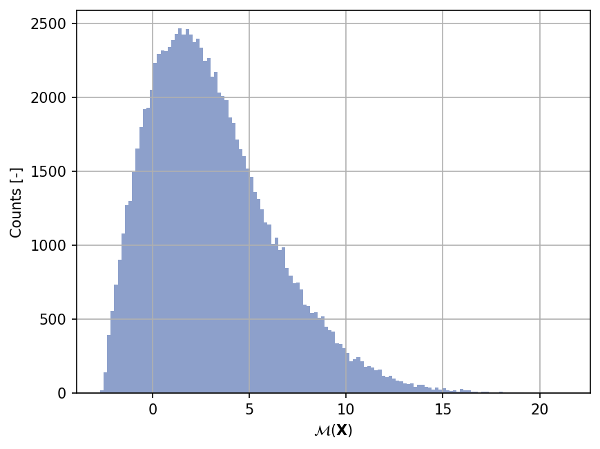
Sample histogram#
Shown below is the histogram of the output based on \(100'000\) random points:
Show code cell source
np.random.seed(42)
xx_test = my_testfun.prob_input.get_sample(100000)
yy_test = my_testfun(xx_test)

plt.hist(yy_test, bins="auto", color="#8da0cb");
plt.grid();
plt.ylabel("Counts [-]");
plt.xlabel("$\mathcal{M}(\mathbf{X})$");
plt.gcf().set_dpi(150);
Sensitivity indices#
The values of \(p\), \(\alpha\) ,and \(\beta\) in the above equation are chosen such that the following conditions are satisfied:
and
where \(S_i\) and \(ST_i\) are the main-effect and total-effect indices for \(i\)-th input variable; and \(\mathbb{V}[Y]\) is the output variance.
References#
Xifu Sun, Barry Croke, Anthony Jakeman, and Stephen Roberts. Benchmarking Active Subspace methods of global sensitivity analysis against variance-based Sobol’ and Morris methods with established test functions. Environmental Modelling & Software, 149:105310, 2022. doi:10.1016/j.envsoft.2022.105310.
Akira Horiguchi, Matthew T. Pratola, and Thomas J. Santner. Assessing variable activity for Bayesian regression trees. Reliability Engineering & System Safety, 207:107391, March 2021. doi:10.1016/j.ress.2020.107391.