Sobol’-G* Function

The Sobol’-G* function (also known as the modified Sobol’-G function) is an \(M\)-dimensional scalar-valued function. It was used in [SAA+10, SCJR22] for testing sensitivity analysis methods.

This function introduces shift and curvature parameters to the original Sobol’-G test function [SSobol95][1].

import numpy as np
import matplotlib.pyplot as plt
import uqtestfuns as uqtf

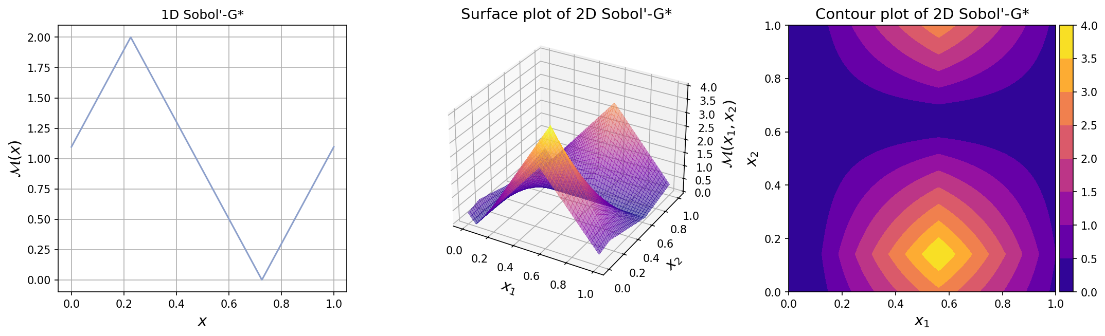
The plots for one-dimensional and two-dimensional Sobol’-G* function are shown below.

Test function instance

To create a default instance of the Sobol’-G* test function, type:

my_testfun = uqtf.SobolGStar()

Check if it has been correctly instantiated:

print(my_testfun)

Function ID      : SobolGStar
Input Dimension  : 2 (variable)
Output Dimension : 1
Parameterized    : True
Description      : Sobol'-G* function from Saltelli et al. (2010)
Applications     : sensitivity

By default, the input dimension is set to \(2\)[2]. To create an instance with another value of input dimension, pass an integer to the parameter input_dimension (the first parameter). For example, to create an instance of the Sobol’-G* function in ten dimensions, type:

my_testfun = uqtf.SobolGStar(input_dimension=10)

In the subsequent section, the function will be illustrated using ten dimensions as it originally appeared in [SAA+10].

Description

The Sobol’-G* function is defined as follows[3]:

\[ \mathcal{M}(\boldsymbol{x}; \boldsymbol{a}, \boldsymbol{\delta}, \boldsymbol{\alpha}) = \prod_{m = 1}^M g^*_m(x_i; a_i, \delta_i, \alpha_i) \]

where

\[ g^*_m(x_i; a_i, \delta_i, \alpha_i) = \frac{(1 + \alpha_i) \lvert 2 (x_i + \delta_i - \lfloor x_i + \delta_i \rfloor) - 1 \rvert^{\alpha_i} + a_i}{1 + a_i} \]

where \(\boldsymbol{x} = \{ x_1, \ldots, x_M \}\) is the \(M\)-dimensional vector of input variables further defined below, and \(\boldsymbol{a}\), \(\boldsymbol{\delta}\), and \(\boldsymbol{\alpha}\) are the parameters of the function further defined below.

Probabilistic input

The probabilistic input model for the Sobol’-G* function consists of \(M\) independent uniform random variables with the ranges shown in the table below.

Show code cell source Hide code cell source

print(my_testfun.prob_input)

Function ID     : SobolGStar
Input ID        : Saltelli2010
Input Dimension : 10
Description     : Probabilistic input model for the Sobol'-G* function from
                  Saltelli et al. (2010)
Marginals       :

 No.    Name    Distribution    Parameters    Description
-----  ------  --------------  ------------  -------------
  1      X1       uniform        [0. 1.]           -
  2      X2       uniform        [0. 1.]           -
  3      X3       uniform        [0. 1.]           -
  4      X4       uniform        [0. 1.]           -
  5      X5       uniform        [0. 1.]           -
  6      X6       uniform        [0. 1.]           -
  7      X7       uniform        [0. 1.]           -
  8      X8       uniform        [0. 1.]           -
  9      X9       uniform        [0. 1.]           -
 10     X10       uniform        [0. 1.]           -

Copulas         : Independence

Parameters

The parameters of the Sobol-G* function—namely the coefficients \(\boldsymbol{a}\), the shift parameter \(\boldsymbol{\delta}\), and the curvature parameter \(\boldsymbol{\alpha}\)—determine the overall behavior of the function. It is worth noting that in the computation of moments and Sobol’ sensitivity indices computation, the shift parameter \(\boldsymbol{\delta}\) has no effect, as it cancels out. This property justifies why the value of \(\boldsymbol{\delta}\) is typically generated randomly.

The available parameters for the Sobol’-G* function are shown in the table below.

Table 8 Parameters of the Sobol’-G* function

No.	\(\boldsymbol{a}\)	\(\boldsymbol{\delta}\)	\(\boldsymbol{\alpha}\)	Keyword	Source	Remark
1.	\(a_1 = a_2 = 0\) \(a_3 = \ldots = 9\)	\(\delta_i \sim \mathcal{U}[0, 1]\)	\(\alpha_i = 1.0\)	Saltelli2010-1 (default)	[SAA+10] (Table 5, test case 1)	Low effective dimension
2.	\(a_i = 0.1 (i - 1), 1 \leq i \leq 5\) \(a_6 = 0.8\) \(a_i = (i - 6), 7 \leq i \leq M\)	\(\delta_i \sim \mathcal{U}[0, 1]\)	\(\alpha_i = 1.0\)	Saltelli2010-2	[SAA+10] (Table 5, test case 2)	High effective dimension
3.	\(a_1 = a_2 = 0\) \(a_3 = \ldots = 9\)	\(\delta_i \sim \mathcal{U}[0, 1]\)	\(\alpha_i = 0.5\)	Saltelli2010-3	[SAA+10] (Table 5, test case 3)	Convex version of 1
4.	\(a_i = 0.1 (i - 1), 1 \leq i \leq 5\) \(a_6 = 0.8\) \(a_i = (i - 6), 7 \leq i \leq M\)	\(\delta_i \sim \mathcal{U}[0, 1]\)	\(\alpha_i = 0.5\)	Saltelli2010-4	[SAA+10] (Table 5, test case 4)	Convex version of 2
5.	\(a_1 = a_2 = 0\) \(a_3 = \ldots = 9\)	\(\delta_i \sim \mathcal{U}[0, 1]\)	\(\alpha_i = 2.0\)	Saltelli2010-5	[SAA+10] (Table 5, test case 5)	Concave version of 1
6.	\(a_i = 0.1 (i - 1), 1 \leq i \leq 5\) \(a_6 = 0.8\) \(a_i = (i - 6), 7 \leq i \leq M\)	\(\delta_i \sim \mathcal{U}[0, 1]\)	\(\alpha_i = 2.0\)	Saltelli2010-6	[SAA+10] (Table 5, test case 6)	Concave version of 2

The default parameter is shown below.

Show code cell source Hide code cell source

print(my_testfun.parameters)

Function ID  : SobolGStar
Parameter ID : Saltelli2010-1
Description  : Parameter set for the Sobol-G* function from Saltelli et
               al.(2010), test case 1; low-effective dimension, easier
               than test case 2

 No.    Keyword      Value      Type        Description
-----  ---------  -----------  -------  -------------------
  1       aa      (10,) array  ndarray   Coefficients 'a'
  2      delta    (10,) array  ndarray    Shift parameter
  3      alpha    (10,) array  ndarray  Curvature parameter

Note

To create an instance of the Sobol’-G* function with a different set of built-in parameters, pass the corresponding keyword to the parameter parameters_id. For example, to use the parameters of test case 2 from [SAA+10], type:

my_testfun = uqtf.SobolGStar(parameters_id="Saltelli2010-2")

Note

The parameter \(\boldsymbol{\delta}\) is randomly generated from a uniform distribution in \([0, 1]^M\) following [SAA+10] when an instance of the function is created; creating a new instance generates a new set of \(\boldsymbol{\delta}\). This parameter cancels out when relevant uncertainty quantification quantities of interest are computed (e.g., variance, sensitivity indices).

To have control over the value of \(\boldsymbol{\delta}\), you can set the value after an instance is created by assigning a set of new values to my_fun.parameters["delta"].

Reference results

This section provides several reference results of typical UQ analyses involving the test function.

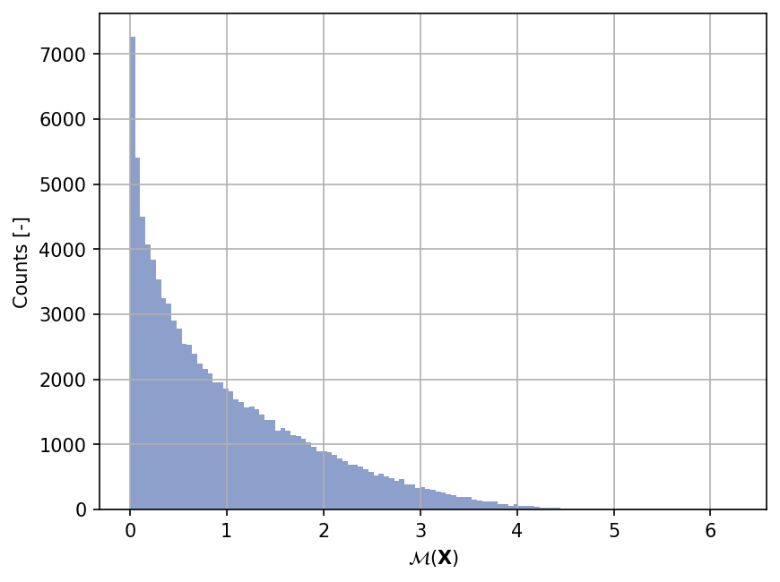
Sample histogram

Shown below is the histogram of the output based on \(100'000\) random points:

Show code cell source Hide code cell source

np.random.seed(42)
xx_test = my_testfun.prob_input.get_sample(100000)
yy_test = my_testfun(xx_test)

plt.hist(yy_test, bins="auto", color="#8da0cb");
plt.grid();
plt.ylabel("Counts [-]");
plt.xlabel("$\mathcal{M}(\mathbf{X})$");
plt.gcf().set_dpi(150);

Definite integration

The integral value of the function over the whole domain \([0, 1]^M\) is analytical:

\[ \int_{[0, 1]^M} \mathcal{M}(\boldsymbol{x}) \; d\boldsymbol{x} = 1.0. \]

Moments estimation

The mean and variance of the Sobol’-G function can be computed analytically.

The mean[4] is given as follows:

\[ \mathbb{E}[Y] = 1.0, \]

while the variance is given as follows:

\[ \mathbb{V}[Y] = \prod_{i = 1}^M (1 + V_i) - 1, \]

where

\[ V_i \equiv \mathbb{V}_{X_i} (\mathbb{E}_{\sim \boldsymbol{X}_i} (Y | X_i)) = \frac{\alpha_i^2}{(1 + 2 \alpha_i) (1 + a_i)^2}. \]

Notice that the value of the variance depend on the choice of the parameter values.

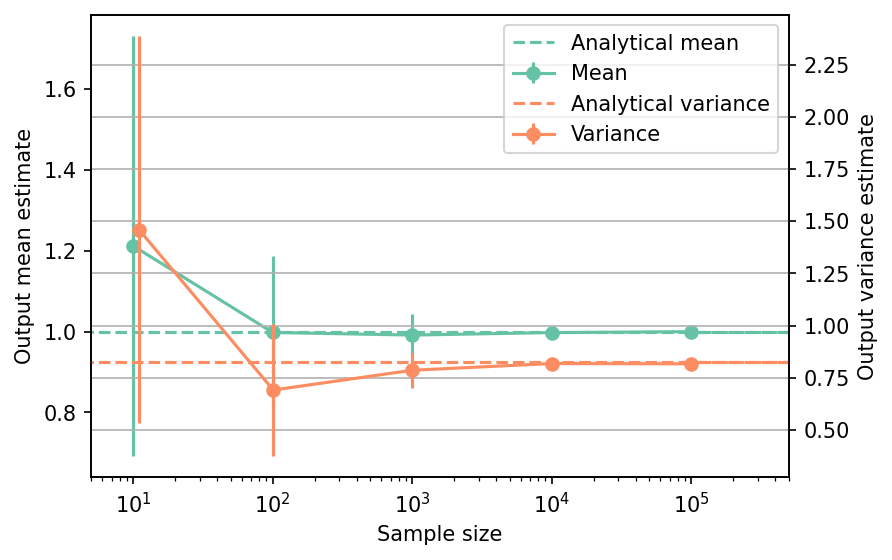
Shown below is the convergence of a direct Monte-Carlo estimation of the output mean and variance with increasing sample sizes compared with the analytical values. The error bars correspond to twice the standard deviation of the estimates obtained from \(50\) replications.

Show code cell source Hide code cell source

# --- Compute the mean and variance estimate
np.random.seed(42)
sample_sizes = np.array([1e1, 1e2, 1e3, 1e4, 1e5], dtype=int)
mean_estimates = np.empty((len(sample_sizes), 50))
var_estimates = np.empty((len(sample_sizes), 50))

for i, sample_size in enumerate(sample_sizes):
    for j in range(50):
        xx_test = my_testfun.prob_input.get_sample(sample_size)
        yy_test = my_testfun(xx_test)
        mean_estimates[i, j] = np.mean(yy_test)
        var_estimates[i, j] = np.var(yy_test)

mean_estimates_errors = np.std(mean_estimates, axis=1)
var_estimates_errors = np.std(var_estimates, axis=1)

# --- Compute analytical mean and variance
mean_analytical = 1.0
aa = my_testfun.parameters["aa"]
alpha = my_testfun.parameters["alpha"]
vv = alpha**2 / (1 + 2 * alpha) / (1 + aa)**2
var_analytical = np.prod(1 + vv) - 1

# --- Plot the mean and variance estimates
fig, ax_1 = plt.subplots(figsize=(6,4))

ext_sample_sizes = np.insert(sample_sizes, 0, 1)
ext_sample_sizes = np.insert(ext_sample_sizes, -1, 5e6)

# --- Mean plot
ax_1.errorbar(
    sample_sizes,
    mean_estimates[:,0],
    yerr=2.0*mean_estimates_errors,
    marker="o",
    color="#66c2a5",
    label="Mean"
)
# Plot the analytical mean
ax_1.plot(
    ext_sample_sizes,
    np.repeat(mean_analytical, len(ext_sample_sizes)),
    linestyle="--",
    color="#66c2a5",
    label="Analytical mean",
)
ax_1.set_xlim([5, 5e5])
ax_1.set_xlabel("Sample size")
ax_1.set_ylabel("Output mean estimate")
ax_1.set_xscale("log");
ax_2 = ax_1.twinx()

# --- Variance plot
ax_2.errorbar(
    sample_sizes+1,
    var_estimates[:,0],
    yerr=2.0*var_estimates_errors,
    marker="o",
    color="#fc8d62",
    label="Variance",
)
# Plot the analytical variance
ax_2.plot(
    ext_sample_sizes,
    np.repeat(var_analytical, len(ext_sample_sizes)),
    linestyle="--",
    color="#fc8d62",
    label="Analytical variance",
)
ax_2.set_ylabel("Output variance estimate")

# Add the two plots together to have a common legend
ln_1, labels_1 = ax_1.get_legend_handles_labels()
ln_2, labels_2 = ax_2.get_legend_handles_labels()
ax_2.legend(ln_1 + ln_2, labels_1 + labels_2, loc=0)

plt.grid()
fig.set_dpi(150)

The tabulated results for each sample size is shown below.

Show code cell source Hide code cell source

from tabulate import tabulate

# --- Compile data row-wise
outputs = [
    [
        np.nan,
        mean_analytical,
        0.0,
        var_analytical,
        0.0,
        "Analytical",
    ]
]

for (
    sample_size,
    mean_estimate,
    mean_estimate_error,
    var_estimate,
    var_estimate_error,
) in zip(
    sample_sizes,
    mean_estimates[:,0],
    2.0*mean_estimates_errors,
    var_estimates[:,0],
    2.0*var_estimates_errors,
):
    outputs += [
        [
            sample_size,
            mean_estimate,
            mean_estimate_error,
            var_estimate,
            var_estimate_error,
            "Monte-Carlo",
        ],
    ]

header_names = [
    "Sample size",
    "Mean",
    "Mean error",
    "Variance",
    "Variance error",
    "Remark",
]

tabulate(
    outputs,
    numalign="center",
    stralign="center",
    tablefmt="html",
    floatfmt=(".1e", ".4e", ".4e", ".4e", ".4e", "s"),
    headers=header_names
)

Sample size	Mean	Mean error	Variance	Variance error	Remark
nan	1.0000e+00	0.0000e+00	8.2574e-01	0.0000e+00	Analytical
1.0e+01	1.2116e+00	5.1889e-01	1.4599e+00	9.2753e-01	Monte-Carlo
1.0e+02	9.9762e-01	1.8848e-01	6.9167e-01	3.1524e-01	Monte-Carlo
1.0e+03	9.9117e-01	5.0990e-02	7.8647e-01	8.4033e-02	Monte-Carlo
1.0e+04	9.9735e-01	1.6111e-02	8.1866e-01	2.4970e-02	Monte-Carlo
1.0e+05	9.9959e-01	6.0113e-03	8.1717e-01	8.2568e-03	Monte-Carlo

Sensitivity indices

The main-effect Sobol’ sensitivity indices of the Sobol’-G* function are given by the following formula:

\[ S_i \equiv \frac{V_i}{\mathbb{V}[Y]}, \; i = 1, \ldots, M, \]

where

\[ \mathbb{V}[Y] = \prod_{i = 1}^M (1 + V_i) - 1, \]

and

\[ V_i = \frac{\alpha_i^2}{(1 + 2 \alpha_i) (1 + a_i)^2}. \]

The total-effect Sobol’ sensitivity indices, on the other hand, are given by the following formula:

\[ ST_i \equiv \frac{VT_i}{\mathbb{V}[Y]}, \; i = 1, \ldots, M, \]

where

\[ VT_i = V_i \prod_{j = 1, j \neq i}^M (1 + V_j). \]

Some example values of the Sobol’ main- and total-effect sensitivity indices for \(10\)-dimensional Sobol’-G* test function are shown in the table below.

Saltelli2010-1

Input	\(S_i\)	\(ST_i\)
\(X_1\)	\(4.03677 \times 10^{-1}\)	\(5.52758 \times 10^{-1}\)
\(X_2\)	\(4.03677 \times 10^{-1}\)	\(5.52758 \times 10^{-1}\)
\(X_3\)	\(4.03677 \times 10^{-3}\)	\(7.34562 \times 10^{-3}\)
\(X_4\)	\(4.03677 \times 10^{-3}\)	\(7.34562 \times 10^{-3}\)
\(X_5\)	\(4.03677 \times 10^{-3}\)	\(7.34562 \times 10^{-3}\)
\(X_6\)	\(4.03677 \times 10^{-3}\)	\(7.34562 \times 10^{-3}\)
\(X_7\)	\(4.03677 \times 10^{-3}\)	\(7.34562 \times 10^{-3}\)
\(X_8\)	\(4.03677 \times 10^{-3}\)	\(7.34562 \times 10^{-3}\)
\(X_9\)	\(4.03677 \times 10^{-3}\)	\(7.34562 \times 10^{-3}\)
\(X_{10}\)	\(4.03677 \times 10^{-3}\)	\(7.34562 \times 10^{-3}\)

Saltelli2010-2

Input	\(S_i\)	\(ST_i\)
\(X_1\)	\(1.20759 \times 10^{-1}\)	\(3.40569 \times 10^{-1}\)
\(X_2\)	\(9.98008 \times 10^{-2}\)	\(2.94228 \times 10^{-1}\)
\(X_3\)	\(8.38604 \times 10^{-2}\)	\(2.56067 \times 10^{-1}\)
\(X_4\)	\(7.14550 \times 10^{-2}\)	\(2.24428 \times 10^{-1}\)
\(X_5\)	\(6.16117 \times 10^{-2}\)	\(1.98005 \times 10^{-1}\)
\(X_6\)	\(3.72713 \times 10^{-2}\)	\(1.27078 \times 10^{-1}\)
\(X_7\)	\(3.01897 \times 10^{-2}\)	\(1.04791 \times 10^{-1}\)
\(X_8\)	\(1.34177 \times 10^{-2}\)	\(4.86527 \times 10^{-2}\)
\(X_9\)	\(7.54743 \times 10^{-3}\)	\(2.78016 \times 10^{-2}\)
\(X_{10}\)	\(4.83036 \times 10^{-3}\)	\(1.79247 \times 10^{-2}\)

Saltelli2010-3

Input	\(S_i\)	\(ST_i\)
\(X_1\)	\(4.49096 \times 10^{-1}\)	\(5.10308 \times 10^{-1}\)
\(X_2\)	\(4.49096 \times 10^{-1}\)	\(5.10308 \times 10^{-1}\)
\(X_3\)	\(4.49096 \times 10^{-3}\)	\(5.73380 \times 10^{-3}\)
\(X_4\)	\(4.49096 \times 10^{-3}\)	\(5.73380 \times 10^{-3}\)
\(X_5\)	\(4.49096 \times 10^{-3}\)	\(5.73380 \times 10^{-3}\)
\(X_6\)	\(4.49096 \times 10^{-3}\)	\(5.73380 \times 10^{-3}\)
\(X_7\)	\(4.49096 \times 10^{-3}\)	\(5.73380 \times 10^{-3}\)
\(X_8\)	\(4.49096 \times 10^{-3}\)	\(5.73380 \times 10^{-3}\)
\(X_9\)	\(4.49096 \times 10^{-3}\)	\(5.73380 \times 10^{-3}\)
\(X_{10}\)	\(4.49096 \times 10^{-3}\)	\(5.73380 \times 10^{-3}\)

Saltelli2010-4

Input	\(S_i\)	\(ST_i\)
\(X_1\)	\(1.79845 \times 10^{-1}\)	\(2.70974 \times 10^{-1}\)
\(X_2\)	\(1.48633 \times 10^{-1}\)	\(2.28349 \times 10^{-1}\)
\(X_3\)	\(1.24893 \times 10^{-1}\)	\(1.94789 \times 10^{-1}\)
\(X_4\)	\(1.06417 \times 10^{-1}\)	\(1.67959 \times 10^{-1}\)
\(X_5\)	\(9.17578 \times 10^{-2}\)	\(1.46209 \times 10^{-1}\)
\(X_6\)	\(5.55078 \times 10^{-2}\)	\(9.05930 \times 10^{-2}\)
\(X_7\)	\(4.49613 \times 10^{-2}\)	\(7.39019 \times 10^{-2}\)
\(X_8\)	\(1.99828 \times 10^{-2}\)	\(3.34077 \times 10^{-2}\)
\(X_9\)	\(1.12403 \times 10^{-2}\)	\(1.89051 \times 10^{-2}\)
\(X_{10}\)	\(7.19381 \times 10^{-3}\)	\(1.21331 \times 10^{-2}\)

Saltelli2010-5

Input	\(S_i\)	\(ST_i\)
\(X_1\)	\(3.26097 \times 10^{-1}\)	\(6.25609 \times 10^{-1}\)
\(X_2\)	\(3.26097 \times 10^{-1}\)	\(6.25609 \times 10^{-1}\)
\(X_3\)	\(3.26097 \times 10^{-3}\)	\(1.11716 \times 10^{-2}\)
\(X_4\)	\(3.26097 \times 10^{-3}\)	\(1.11716 \times 10^{-2}\)
\(X_5\)	\(3.26097 \times 10^{-3}\)	\(1.11716 \times 10^{-2}\)
\(X_6\)	\(3.26097 \times 10^{-3}\)	\(1.11716 \times 10^{-2}\)
\(X_7\)	\(3.26097 \times 10^{-3}\)	\(1.11716 \times 10^{-2}\)
\(X_8\)	\(3.26097 \times 10^{-3}\)	\(1.11716 \times 10^{-2}\)
\(X_9\)	\(3.26097 \times 10^{-3}\)	\(1.11716 \times 10^{-2}\)
\(X_{10}\)	\(3.26097 \times 10^{-3}\)	\(1.11716 \times 10^{-2}\)

Saltelli2010-6

Input	\(S_i\)	\(ST_i\)
\(X_1\)	\(4.98832 \times 10^{-2}\)	\(4.72157 \times 10^{-1}\)
\(X_2\)	\(4.12258 \times 10^{-2}\)	\(4.22827 \times 10^{-1}\)
\(X_3\)	\(3.46411 \times 10^{-2}\)	\(3.79412 \times 10^{-1}\)
\(X_4\)	\(2.95167 \times 10^{-2}\)	\(3.41319 \times 10^{-1}\)
\(X_5\)	\(2.54506 \times 10^{-2}\)	\(3.07929 \times 10^{-1}\)
\(X_6\)	\(1.53961 \times 10^{-2}\)	\(2.10367 \times 10^{-1}\)
\(X_7\)	\(1.24708 \times 10^{-2}\)	\(1.77059 \times 10^{-1}\)
\(X_8\)	\(5.54258 \times 10^{-3}\)	\(8.67228 \times 10^{-2}\)
\(X_9\)	\(3.11770 \times 10^{-3}\)	\(5.05883 \times 10^{-2}\)
\(X_{10}\)	\(1.99533 \times 10^{-3}\)	\(3.29412 \times 10^{-2}\)

References

[SSobol95]

Andrea Saltelli and Ilya M. Sobol'. About the use of rank transformation in sensitivity analysis of model output. Reliability Engineering & System Safety, 50(3):225–239, 1995. doi:10.1016/0951-8320(95)00099-2.

[SAA+10] (1,2,3,4,5,6,7,8,9,10,11)

Andrea Saltelli, Paola Annoni, Ivano Azzini, Francesca Campolongo, Marco Ratto, and Stefano Tarantola. Variance based sensitivity analysis of model output. design and estimator for the total sensitivity index. Computer Physics Communications, 181(2):259–270, 2010. doi:10.1016/j.cpc.2009.09.018.

[SCJR22]

Xifu Sun, Barry Croke, Anthony Jakeman, and Stephen Roberts. Benchmarking Active Subspace methods of global sensitivity analysis against variance-based Sobol’ and Morris methods with established test functions. Environmental Modelling & Software, 149:105310, 2022. doi:10.1016/j.envsoft.2022.105310.

---

[1]

In particular, to avoid unfair advantage to a design of experiment where the mid-point of the domain is discontinuous in the original formula.

[2]

This default dimension applies to all variable dimension test functions. It will be used if the input_dimension argument is not given.

[3]

see Eqs. (27) and (28), p. 265 in [SAA+10].

[4]

The expected value is the same as the integral over the domain because the input is uniform in a unit hypercube.