Sine Function from Currin et al. (1988)#
import numpy as np
import matplotlib.pyplot as plt
import uqtestfuns as uqtf
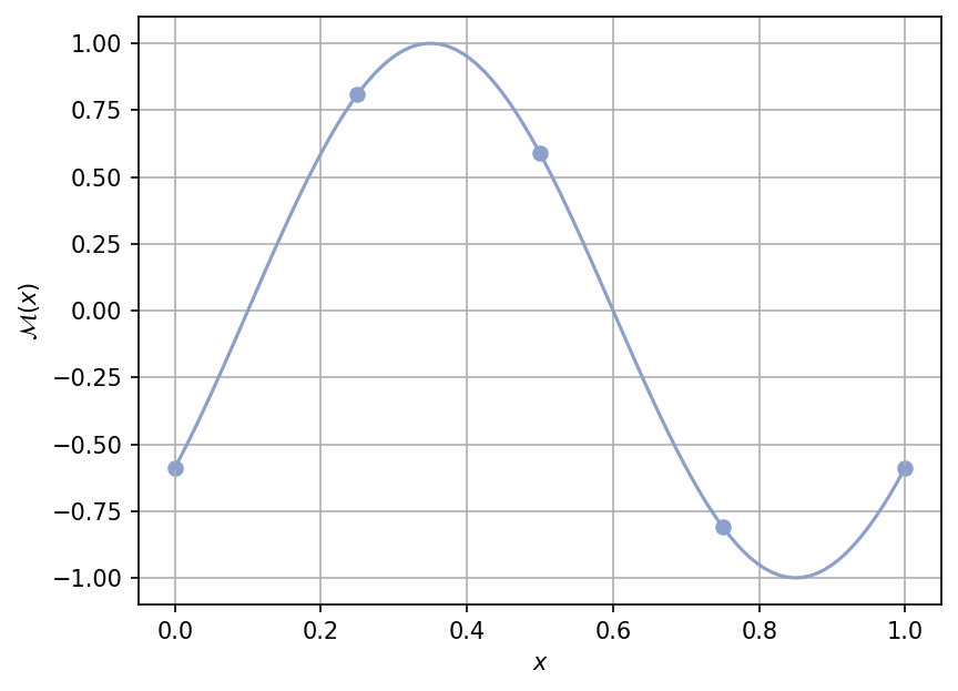
The function is a simple one-dimensional, scalar-valued test function. It was featured in [CMMY88] as an example introducing Gaussian process metamodeling method.
A plot of the function is shown below..
Note
In the original paper, the function was evaluated at \(x = \{ 0.00, 0.25, 0.50, 0.75, 1.00 \}\) to serve as the training data; these points are shown in the above plot.
Test function instance#
To create a default instance of the test function:
my_testfun = uqtf.CurrinSine()
Check if it has been correctly instantiated:
print(my_testfun)
Function ID      : CurrinSine
Input Dimension  : 1 (fixed)
Output Dimension : 1
Parameterized    : False
Description      : Sine function from Currin et al. (1988)
Applications     : metamodeling
Description#
The test function is analytically defined as follows[1]:
where \(x\) is further defined below.
Probabilistic input#
The probabilistic input model for the test function is shown below.
Show code cell source
print(my_testfun.prob_input)
Function ID     : CurrinSine
Input ID        : Currin1988
Input Dimension : 1
Description     : Input model for the Sine function from Currin et al.
                  (1988)
Marginals       :

 No.    Name    Distribution    Parameters    Description
-----  ------  --------------  ------------  -------------
  1      x        uniform        [0. 1.]           -
Reference results#
This section provides several reference results of typical UQ analyses involving the test function.
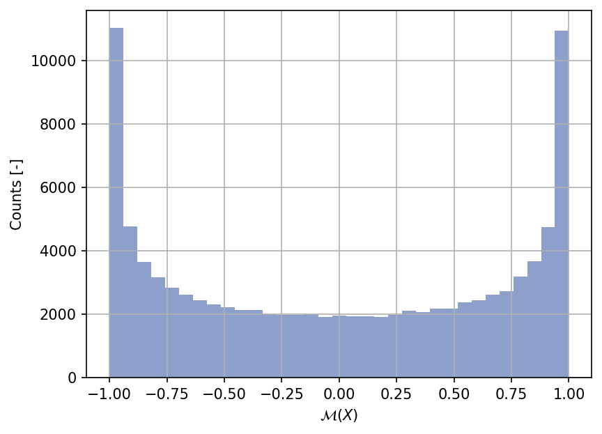
Sample histogram#
Shown below is the histogram of the output based on \(100'000\) random points:
Show code cell source
my_testfun.prob_input.reset_rng(42)
xx_test = my_testfun.prob_input.get_sample(100000)
yy_test = my_testfun(xx_test)

plt.hist(yy_test, bins="auto", color="#8da0cb");
plt.grid();
plt.ylabel("Counts [-]");
plt.xlabel("$\mathcal{M}(X)$");
plt.gcf().tight_layout(pad=3.0)
plt.gcf().set_dpi(150);
References#
C. Currin, T. Mitchell, M. Morris, and D. Ylvisaker. A Bayesian approach to the design and analysis of computer experiments. Technical Report ORNL-6498, Oak Ridge National Laboratory, Oak Ridge, Tennessee, 1988. doi:10.2172/814584.