Linear Function from Linkletter et al. (2006)#
import numpy as np
import matplotlib.pyplot as plt
import uqtestfuns as uqtf
The function is a ten-dimensional, scalar-valued function. Only the first four input variables are active, while the rest is inert. The function was used in [LBH+06] to demonstrate a variable selection method (i.e., sensitivity analysis) in the context of Gaussian process metamodeling.
Note
Linkletter et al. [LBH+06] introduced four ten-dimensional analytical test functions with some of the input variables inert. They are used to demonstrate a variable selection method (i.e., screening) in the context of Gaussian process metamodeling:
Linear function features a simple function with four active input variables (out of 10). (this function)
Linear with decreasing coefficients function features a slightly more complex linear function with eight active input variables (out of 10).
Sine function features only two active input variables (out of 10); the effect of the two inputs on the output, however, is very different.
Inert function does not have any active input variables; a constant zero is returned for any input values.
Test function instance#
To create a default instance of the test function:
my_testfun = uqtf.LinkletterLinear()
Check if it has been correctly instantiated:
print(my_testfun)
Function ID      : LinkletterLinear
Input Dimension  : 10 (fixed)
Output Dimension : 1
Parameterized    : False
Description      : Linear function with 4 active inputs from Linkletter et al. (2006)
Applications     : metamodeling, sensitivity
Description#
The test function is defined as[1]:
where \(\boldsymbol{x} = \left( x_1, \ldots x_{10} \right)\) is the ten-dimensional vector of input variables further defined below. Notice that only four out of ten input variables are active.
Note
In the original paper, the function was added with an independent identically distributed (i.i.d) noise from \(\mathcal{N}(0, \sigma)\) with a standard deviation \(\sigma = 0.05\).
Furthermore, also in the original paper, a batch of data is generated from the function and then standardized to have mean \(0.0\) and standard deviation \(1.0\).
The implementation of UQTestFuns does not include any error addition or standardization. However, these processes can be done manually after the data is generated.
Probabilistic input#
The probabilistic input model for the test function is shown below.
Show code cell source
print(my_testfun.prob_input)
Function ID     : LinkletterLinear
Input ID        : Linkletter2006
Input Dimension : 10
Description     : Input specification for the linear test function Eq.
                  (5)from Linkletter et al. (2006)
Marginals       :

 No.    Name    Distribution    Parameters    Description
-----  ------  --------------  ------------  -------------
  1     x_1       uniform         [0 1]            -
  2     x_2       uniform         [0 1]            -
  3     x_3       uniform         [0 1]            -
  4     x_4       uniform         [0 1]            -
  5     x_5       uniform         [0 1]            -
  6     x_6       uniform         [0 1]            -
  7     x_7       uniform         [0 1]            -
  8     x_8       uniform         [0 1]            -
  9     x_9       uniform         [0 1]            -
 10     x_10      uniform         [0 1]            -

Copulas         : Independence
Reference results#
This section provides several reference results of typical UQ analyses involving the test function.
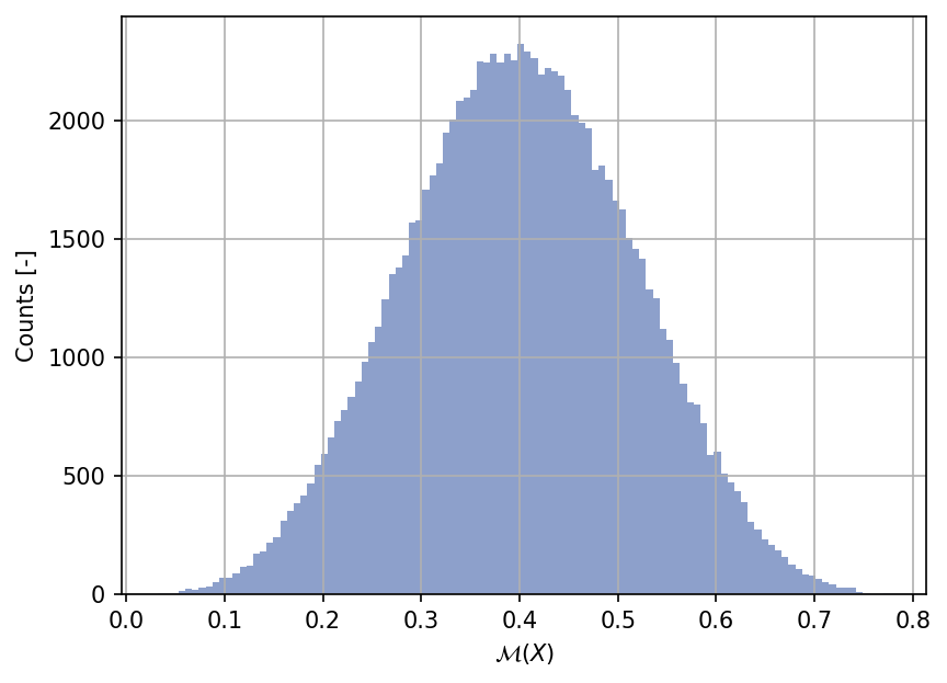
Sample histogram#
Shown below is the histogram of the output based on \(100'000\) random points:
Show code cell source
my_testfun.prob_input.reset_rng(42)
xx_test = my_testfun.prob_input.get_sample(100000)
yy_test = my_testfun(xx_test)

plt.hist(yy_test, bins="auto", color="#8da0cb");
plt.grid();
plt.ylabel("Counts [-]");
plt.xlabel("$\mathcal{M}(X)$");
plt.gcf().tight_layout(pad=3.0)
plt.gcf().set_dpi(150);
References#
Crystal Linkletter, Derek Bingham, Nicholas Hengartner, David Higdon, and Kenny Q. Ye. Variable selection for Gaussian process models in computer experiments. Technometrics, 48(4):478–490, 2006. doi:10.1198/004017006000000228.