Rosenbrock Function#
The Rosenbrock function, originally introduced in [Ros60] as a two-dimensional scalar-valued test function for global optimization, was later generalized to \(M\) dimensions. It has since become a widely used benchmark for global optimization methods (e.g., [DS78, PWG13]). In [Tan15], the function was employed in a metamodeling exercise.
The function is also known as the valley function or the banana function.
import numpy as np
import matplotlib.pyplot as plt
import uqtestfuns as uqtf
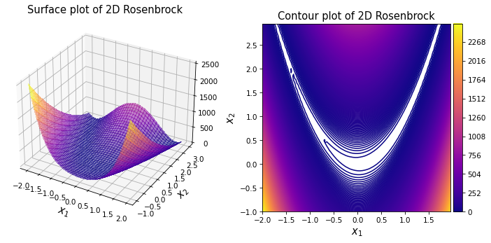
The surface and contour plots for the two-dimensional Rosenbrock function are shown below for the default parameter set and for \(x \in [-2, 2] \times [-1, 3]\).
As shown, the function features a curved, non-convex valley. While it is relatively easy to reach the valley, the convergence to the global minimum is difficult.
Test function instance#
To create a default instance of the test function, type:
my_testfun = uqtf.Rosenbrock()
Check if it has been correctly instantiated:
print(my_testfun)
Function ID      : Rosenbrock
Input Dimension  : 2 (variable)
Output Dimension : 1
Parameterized    : True
Description      : Optimization test function from Rosenbrock (1960), also known as the banana function
Applications     : optimization, metamodeling
By default, the input dimension is set to \(2\)[1].
To create an instance with another value of input dimension,
pass an integer to the parameter input_dimension (keyword only).
For example, to create an instance of 10-dimensional Rosenbrock function, type:
my_testfun = uqtf.Ackley(input_dimension=10)
Description#
The generalized Rosenbrock function is defined as follows:
where \(\boldsymbol{x} = \{ x_1, \ldots, x_M \}\) is the \(M\)-dimensional vector of input variables, as defined below, and \(\boldsymbol{p} = \{ a, b, c, d \}\) is the set of parameters also defined further below.
Input#
The Rosenbrock function is defined on \(\mathbb{R}^M\), but in the context of optimization test function, the search space is often limited as shown in the table below.
Show code cell source
print(my_testfun.prob_input)
Function ID     : Rosenbrock
Input ID        : Picheny2013
Input Dimension : 2
Description     : Search domain for the Rosenbrock function from Picheny et
                  al. (2013)
Marginals       :

 No.    Name    Distribution    Parameters    Description
-----  ------  --------------  ------------  -------------
  1      x1       uniform       [-5. 10.]          -
  2      x2       uniform       [-5. 10.]          -

Copulas         : Independence
Parameters#
The Rosenbrock function requires four additional parameters to complete the specification. The default values are shown below.
Show code cell source
print(my_testfun.parameters)
Function ID  : Rosenbrock
Parameter ID : Rosenbrock1960
Description  : Parameter set for the Rosenbrock function from Rosenbrock
               (1960)

 No.    Keyword      Value      Type                    Description
-----  ---------  -----------  ------  ---------------------------------------------
  1        a      1.00000e+00  float         Global optimum location and value
  2        b      1.00000e+02  float   Steepness, curvature, and width of the valley
  3        c      0.00000e+00  float                  Shift parameter
  4        d      1.00000e+00  float                  Scale parameter
The parameter \(a\) controls the location and value of the global optimum. The parameter \(b\) controls the steepness and width of the valley. In particular, it determines the scale of variation of the function; large value of \(b\) creates a steeper and tight valley.
The parameters \(c\) and \(d\) are used to shift and scale the function such that its mean and standard deviation become \(0.0\) and \(1.0\), respectively.
Below are some contour plots of the function in two dimensions with different values of \(a\) and \(b\) along with the location of the global optimum.
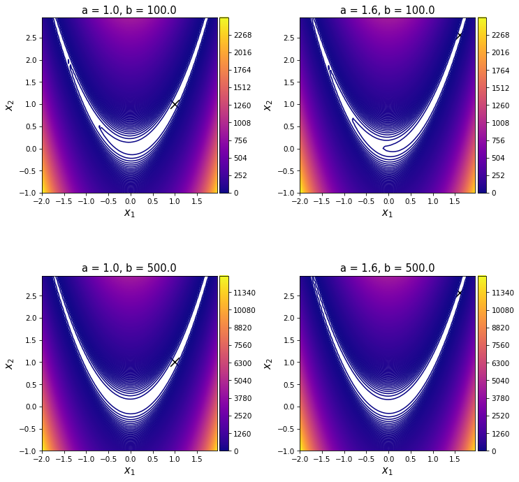
As mentioned earlier, the changing the value of \(a\) modifies the location of the global optimum (and in \(M > 2\) modifies the function value at the optimum). Changing the value of \(b\), on the other hand, modifies the scale of the function variation and the steepness of the valley (see the color bar).
Reference results#
This section provides several reference results related to the test function.
Optimum values#
The global optimum of the Rosenbrock function is located at
In dimension two, the function value at the optimum location is always \(0.0\) (but not in higher dimension!).
References#
L. C. W. Dixon and G. P. Szegö. Towards global optimization 2, chapter The global optimization problem: an introduction, pages 1–15. North-Holland, Amsterdam, 1978.
H. H. Rosenbrock. An automatic method for finding the greatest or least value of a function. The Computer Journal, 3(3):175–184, 1960. doi:10.1093/comjnl/3.3.175.
Victor Picheny, Tobias Wagner, and David Ginsbourger. A benchmark of kriging-based infill criteria for noisy optimization. Structural and Multidisciplinary Optimization, 48(3):607–626, 2013. doi:10.1007/s00158-013-0919-4.
Matthias Hwai Yong Tan. Stochastic polynomial interpolation for uncertainty quantification with computer experiments. Technometrics, 57(4):457–467, 2015. doi:10.1080/00401706.2014.950431.