Welch et al. (1992) Function#
import numpy as np
import matplotlib.pyplot as plt
import uqtestfuns as uqtf
The Welch et al. (1992) test function (or the Welch1992 function for short)
is a 20-dimensional scalar-valued function.
The function features some strong non-linearities as well as some
pair interaction effects. Furthermore, a couple of two input variables
are set to be inert.
The function was introduced in Welch et al. (1992) [WBS+92] as a test function for metamodeling and sensitivity analysis purposes. The function is also suitable for testing multi-dimensional integration algorithms.
Test function instance#
To create a default instance of the test function:
my_testfun = uqtf.Welch1992()
Check if it has been correctly instantiated:
print(my_testfun)
Function ID      : Welch1992
Input Dimension  : 20 (fixed)
Output Dimension : 1
Parameterized    : False
Description      : 20-Dimensional function from Welch et al. (1992)
Applications     : metamodeling, sensitivity, integration
Description#
The Welch1992 function is defined as follows[1]:
where \(\boldsymbol{x} = \{ x_1, \ldots, x_{20} \}\) is the 20-dimensional vector of input variables further defined below. Notice that the input variables \(x_8\) and \(x_{16}\) are inert and therefore, missing from the expression.
Probabilistic input#
Based on [WBS+92], the test function is defined on the 20-dimensional input space \([-0.5, 0.5]^{20}\). This input can be modeled using 20 independent uniform random variables shown in the table below.
Show code cell source
print(my_testfun.prob_input)
Function ID     : Welch1992
Input ID        : Welch1992
Input Dimension : 20
Description     : Input specification for the test function from Welch et
                  al. (1992)
Marginals       :

 No.    Name    Distribution    Parameters    Description
-----  ------  --------------  ------------  -------------
  1      x1       uniform      [-0.5  0.5]         -
  2      x2       uniform      [-0.5  0.5]         -
  3      x3       uniform      [-0.5  0.5]         -
  4      x4       uniform      [-0.5  0.5]         -
  5      x5       uniform      [-0.5  0.5]         -
  6      x6       uniform      [-0.5  0.5]         -
  7      x7       uniform      [-0.5  0.5]         -
  8      x8       uniform      [-0.5  0.5]         -
  9      x9       uniform      [-0.5  0.5]         -
 10     x10       uniform      [-0.5  0.5]         -
 11     x11       uniform      [-0.5  0.5]         -
 12     x12       uniform      [-0.5  0.5]         -
 13     x13       uniform      [-0.5  0.5]         -
 14     x14       uniform      [-0.5  0.5]         -
 15     x15       uniform      [-0.5  0.5]         -
 16     x16       uniform      [-0.5  0.5]         -
 17     x17       uniform      [-0.5  0.5]         -
 18     x18       uniform      [-0.5  0.5]         -
 19     x19       uniform      [-0.5  0.5]         -
 20     x20       uniform      [-0.5  0.5]         -

Copulas         : Independence
Reference Results#
This section provides several reference results of typical analyses involving the test function.
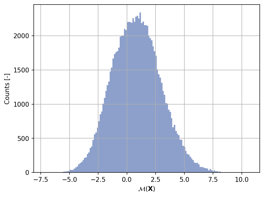
Sample histogram#
Shown below is the histogram of the output based on \(100'000\) random points:
Show code cell source
np.random.seed(42)
xx_test = my_testfun.prob_input.get_sample(100000)
yy_test = my_testfun(xx_test)

plt.hist(yy_test, bins="auto", color="#8da0cb");
plt.grid();
plt.ylabel("Counts [-]");
plt.xlabel("$\mathcal{M}(\mathbf{X})$");
plt.gcf().set_dpi(150);
Definite integration#
The integral value of the test function over the domain \([-0.5, 0.5]^{20}\) is analytical:
Moments estimation#
The moments of the test function may be derived analytically; the first two (i.e., the expected value and the variance) are given below.
Expected value#
Due to the fact that the function domain is a hypercube and the input variables are uniformly distributed, the expected value of the function is the same as the integral value over the domain:
Variance#
The analytical value (albeit inexact) for the variance is given as follows:
References#
William J. Welch, Robert. J. Buck, Jerome Sacks, Henry P. Wynn, Toby J. Mitchell, and Max D. Morris. Screening, predicting, and computer experiments. Technometrics, 34(1):15, 1992. doi:10.2307/1269548.