Uncertainty Quantification Framework#
Consider a computational model that is represented as an \(M\)-dimensional black-box function:
where \(\mathcal{D}_{\boldsymbol{X}}\), \(\boldsymbol{y}\), \(P\) denote the input domain, the quantity of interest (QoI), and the dimensionality of the output space, respectively.
In practice, the exact values of the input variables are often not known exactly and may be considered uncertain. The ensuing analysis involving uncertain input variables can be formalized in the uncertainty quantification (UQ) framework following [Sud07] as illustrated in Fig. 1.
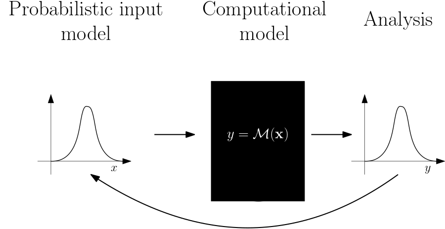
Fig. 1 Uncertainty quantification (UQ) framework, adapted from [Sud07].#
The framework starts from the center, with the computational model \(\mathcal{M}\) taken as a black-box as defined earlier. Then it moves on to the probabilistic modeling of the (uncertain) input variables. Under the probabilistic modeling, the uncertain input variables are represented by a random vector equipped with a joint probability density function (PDF)
Subsequently, the uncertainties of the input variables are propagated through the computational model \(\mathcal{M}\). As a result, the quantity of interest \(\boldsymbol{y}\) now itself becomes a random vector[1]:
This leads to various downstream analyses such as:
reliability analysis: Estimating the probability of small or rare failure events.
sensitivity analysis: Quantifying the contribution of the input uncertainties to output uncertainty.
metamodeling: Constructing a fast surrogate approximation for a typically expensive computational model.
In UQTestFuns, these analyses form the primary categories of UQ test functions based on their applications in the literature[2]. Additionally, many global sensitivity analysis problems reduce to solving an integration problem, which explains the extra category. For completeness, UQTestFuns also includes test functions commonly used for benchmarking testing optimization methods.