Creating a One-Dimensional Marginal Distribution#
A probabilistic input to a UQ test function consists of input variables each of which is a (univariate) random variable. Therefore, the starting point of defining a (possibly multivariate) probabilistic input is defining the distribution for each of the constituent random variables. This page explains how such a marginal distribution can be created in UQTestFuns.
import matplotlib.pyplot as plt
import numpy as np
import uqtestfuns as uqtf
Suppose we would like to define one-dimensional triangular marginal distribution for random variable \(X\):
where \(a\), \(b\), and \(c\) are the parameters of the triangular distribution. These parameters correspond to the lower bound, the upper bound, and the mid-point of the distribution. For this particular example, we set these values to \(3.0\), \(5.0\), and \(4.0\).
A Marginal instance#
A univariate random variable is represented in UQTestFuns by the Marginal class.
To create an instance of the class, you need to pass the following arguments:
distribution: the chosen univariate distribution (one from this list)parameters: the parameters of the distribution (note that the number of required parameters differs from distribution to another)name: the name of the random variable (optional)description: a short text describing the random variable (optional)
To create an instance, type:
my_rand_var = uqtf.Marginal(
    distribution="triangular",
    parameters=[3.0, 5.0, 4.0],
    name="X",
    description="My random variable",
)
my_rand_var
Marginal(distribution='triangular', parameters=array([3., 5., 4.]), name='X', description='My random variable')
The variable my_rand_var now stores an instance
of a univariate random variable distributed as triangular
with the specified parameters.
An instance of Marginal exposes the following properties:
Property |
Description |
|---|---|
|
the assigned name of the random variable (may be |
|
the assigned description of the random variable (may be |
|
the distribution (one of available distributions) |
|
the parameters of the distribution |
|
the lower bound of the distribution |
|
the upper bound of the distribution |
and methods:
Method |
Description |
|---|---|
|
compute the cumulative distribution function on a set of values |
|
compute the probability density function on a set of values |
|
compute the inverse cumulative distribution function on a set of values |
|
get a sample of size |
|
transform a set of sample values |
Let’s go through each one of these methods.
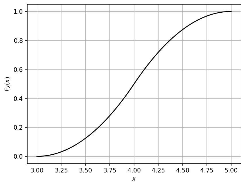
Computing the CDF values#
The CDF values for a set of sample values in \(\mathcal{D}_X\) can be computed using the cdf() method.
Suppose we want to evaluate the CDF of the distribution on its support:
xx = np.linspace(my_rand_var.lower, my_rand_var.upper, 1000)
yy_cdf = my_rand_var.cdf(xx)
The plot is shown below:
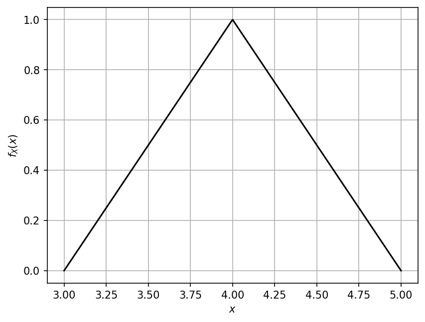
Computing the PDF values#
The PDF values for a set of sample values in \(\mathcal{D}_X\)
can be computed using the pdf() method.
Similarly as before:
yy_pdf = my_rand_var.pdf(xx)
and with the plot shown below.
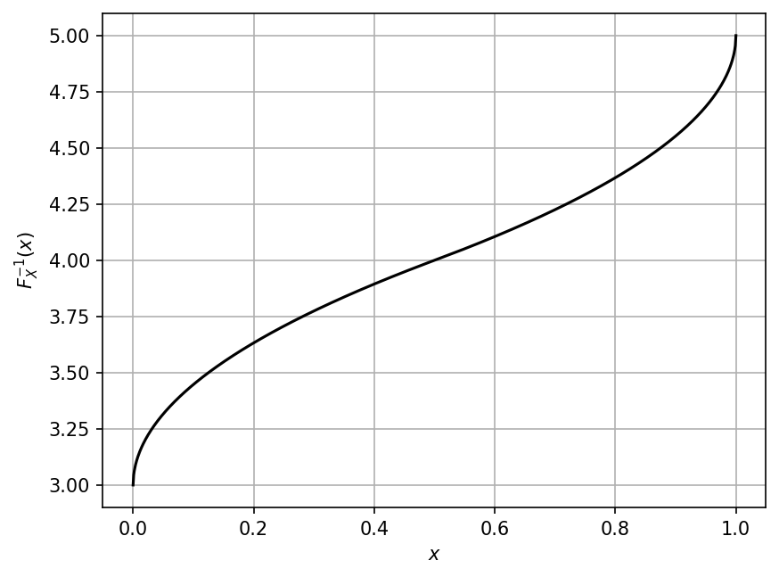
Computing the ICDF values#
The ICDF values can be obtained using the icdf() method.
Unlike the CDF and PDF, the input to ICDF is a probability value \(p\) in \([0, 1]\).
For a given \(p\), the function returns the quantile value,
i.e., the value \(x\) such that \(F_X (x) = \mathbb{P}[X \leq x] = p\)
Suppose we want to compute the ICDF on a set of equidistant points in \([0, 1]\):
xx_icdf = np.linspace(0, 1, 1000)
yy_icdf = my_rand_var.icdf(xx_icdf)
The plot of the ICDF is shown below.
Getting a sample#
Strictly speaking, sampling a random variable \(X\) means generating a value \(x\)
in \(\mathcal{D}_X\) such that the probability of getting \(x\)
is following the distribution \(F_X(x)\).
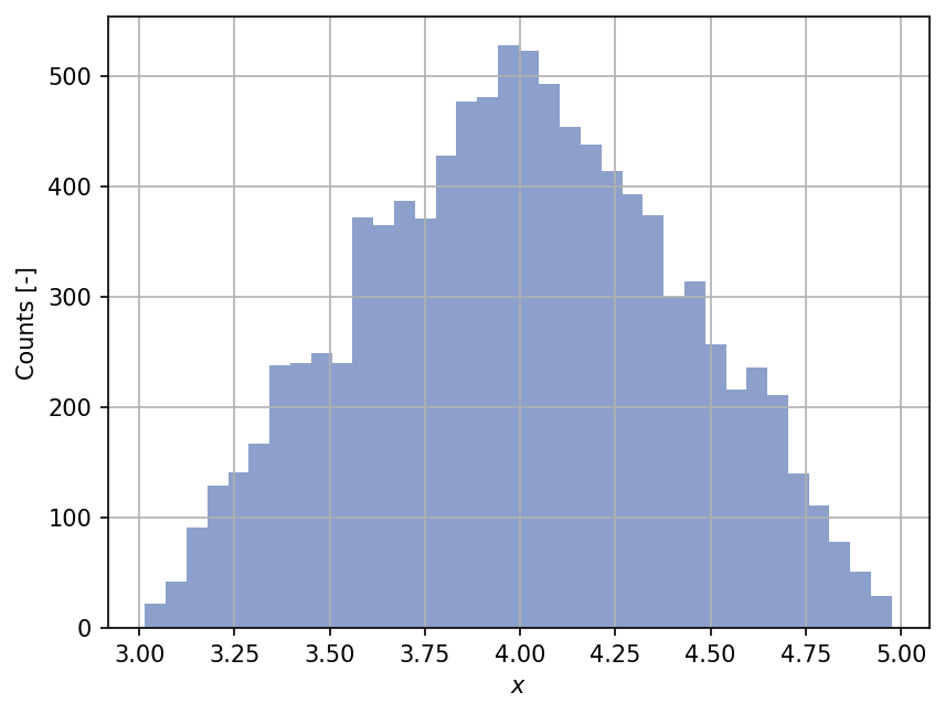
The get_sample() method allows us to generate a sample
of a given size from the random variable.
For instance, in the code below, we generate \(10'000\) sample points:
xx_sample = my_rand_var.get_sample(10000)
To see whether this sample is distributed according to the specified triangular distribution, we can make a histogram of it:
Transforming a sample#
The transform_sample() method facilitates the transformation
between a sample generated from one distribution to another.
Let’s suppose, complementary to the random variable \(X\) we define another random variable as follows:
my_rand_var_2 = uqtf.Marginal(distribution="normal", parameters=[0, 1], name="Y")
In other words, the variable \(Y\) is a standard normal random variable. The sample from \(X\) can be transformed to \(Y\) as follows:
xx_sample_2 = my_rand_var.transform_sample(xx_sample, my_rand_var_2)
---------------------------------------------------------------------------
AttributeError                            Traceback (most recent call last)
Cell In[12], line 1
----> 1 xx_sample_2 = my_rand_var.transform_sample(xx_sample, my_rand_var_2)

AttributeError: 'Marginal' object has no attribute 'transform_sample'
The histogram of the transformed sample is shown below.
Note
The transformation of sample from the standard uniform random variable to another (say, target) random variable is the basis of the so-called inverse transform sampling. This is because the transformation function is the ICDF of the target distribution.
Notes on the support of a distribution#
The support of a univariate continuous random variable consists of two components, the lower and upper bounds. In the case of the above triangular distribution, its support is \(\mathcal{D}_X = [3.0, 5.0]\) (the lower and upper bounds are \(3.0\) and \(5.0\), respectively). Such a distribution is supported on a bounded interval; specifically, the distribution is bounded from the right (below) and left (above).
Consider, on the other hand, the standard normal distribution. Its support is, strictly speaking, \(\mathcal{D}_X = (-\infty, \infty)\). This is an example of distributions that are supported on the whole real line; it is neither bounded from below nor from above.
The properties of a Marginal instance include among other things,
lower (lower bound) and upper (upper bound).
For the triangular distribution defined above, the lower and upper bounds are indeed:
my_rand_var.lower, my_rand_var.upper
However, for the standard normal distribution, they are:
my_rand_var_2.lower, my_rand_var_2.upper
which means that this distribution in UQTestFuns is actually bounded.
This “truncation” is based on practical consideration. Numerically, at least, infinity does not mean much. The distribution must be numerically truncated somehow. In the case of standard normal distribution, the value of \(-8.22\) and \(8.21\) correspond to the quantile values whose probabilities are \(10^{-16}\) and \(1-10^{-16}\), respectively.
This means that by truncating the unbounded standard normal distribution from both sides at these values, we are consciously ignoring the values whose probabilities are at most \(10^{-16}\). This is an acceptable assumption in typical engineering applications.