Ishigami Function#

import numpy as np
import matplotlib.pyplot as plt
import uqtestfuns as uqtf

The Ishigami test function is a three-dimensional scalar-valued function. First introduced in [IH91] in the context of sensitivity analysis, the function has been revisited many times in the same context (see for instances [SobolL99, Sud08, MILR09]).

Test function instance#

To create a default instance of the Ishigami test function:

my_testfun = uqtf.Ishigami()

Check if it has been correctly instantiated:

print(my_testfun)

Name              : Ishigami
Spatial dimension : 3
Description       : Ishigami function from Ishigami and Homma (1991)

Description#

The Ishigami function, a highly non-linear and non-monotonic function, is given as follows:

\[ \mathcal{M}(\boldsymbol{x}) = \sin(x_1) + a \sin^2(x_2) + b \, x_3^4 \sin(x_1) \]

where \(\boldsymbol{x} = \{ x_1, x_2, x_3 \}\) is the three-dimensional vector of input variables further defined below, and \(a\) and \(b\) are parameters of the function.

Probabilistic input#

Based on [IH91], the probabilistic input model for the Ishigami function consists of three independent uniform random variables with the ranges shown in the table below.

my_testfun.prob_input

Name: Ishigami1991

Spatial Dimension: 3

Description: Probabilistic input model for the Ishigami function from Ishigami and Homma (1991).

Marginals:

No.	Name	Distribution	Parameters	Description
1	X1	uniform	[-3.14159265 3.14159265]	None
2	X2	uniform	[-3.14159265 3.14159265]	None
3	X3	uniform	[-3.14159265 3.14159265]	None

Copulas: None

Parameters#

The parameters of the Ishigami function are two real-valued numbers. Some of the available parameter values taken from the literature are shown in the table below.

No.	Value	Keyword	Source
1	\(a = 7\), \(b = 0.1\)	`Ishigami1991` (default)	[IH91]
2	\(a = 7\), \(b = 0.05\)	`Sobol1999`	[SobolL99]

Alternatively, to create an instance of the Ishigami function with different parameter values, type:

my_testfun = uqtf.Ishigami(parameters_selection="Sobol1999")

Note

To use another set of parameters, create a default test function and pass one of the available keywords (as indicated in the table above) to the parameters_selection parameter. For example:

my_testfun = uqtf.Ishigami(parameters_selection="Sobol1999")

Reference results#

This section provides several reference results of typical UQ analyses involving the test function.

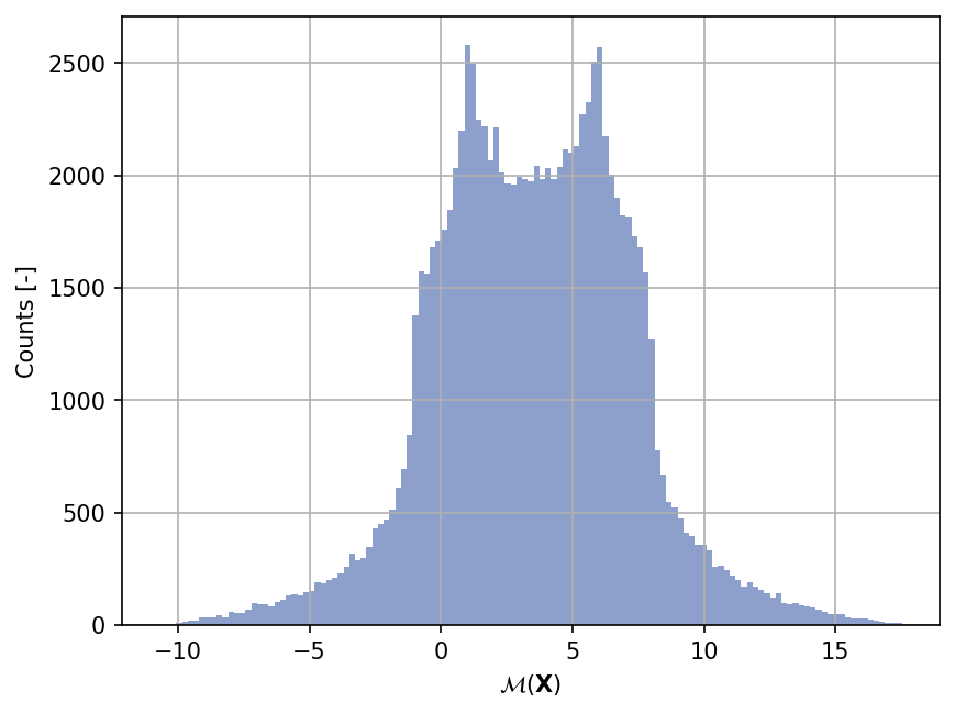
Sample histogram#

Shown below is the histogram of the output based on \(100'000\) random points:

np.random.seed(42)
xx_test = my_testfun.prob_input.get_sample(100000)
yy_test = my_testfun(xx_test)

plt.hist(yy_test, bins="auto", color="#8da0cb");
plt.grid();
plt.ylabel("Counts [-]");
plt.xlabel("$\mathcal{M}(\mathbf{X})$");
plt.gcf().set_dpi(150);

Moment estimations#

The mean and variance of the Ishigami function can be computed analytically,
and the results are:

\(\mathbb{E}[Y] = \frac{a}{2}\)
\(\mathbb{V}[Y] = \frac{a^2}{8} + \frac{b \pi^4}{5} + \frac{b^2 \pi^8}{18} + \frac{1}{2}\)

Notice that the values of these two moments depend on the choice of the parameter values.

Shown below is the convergence of a direct Monte-Carlo estimation of the output mean and variance with increasing sample sizes compared with the analytical values.

# --- Compute the mean and variance estimate
np.random.seed(42)
sample_sizes = np.array([1e1, 1e2, 1e3, 1e4, 1e5, 1e6, 1e7], dtype=int)
mean_estimates = np.empty(len(sample_sizes))
var_estimates = np.empty(len(sample_sizes))

for i, sample_size in enumerate(sample_sizes):
    xx_test = my_testfun.prob_input.get_sample(sample_size)
    yy_test = my_testfun(xx_test)
    mean_estimates[i] = np.mean(yy_test)
    var_estimates[i] = np.var(yy_test)

# --- Compute the error associated with the estimates
mean_estimates_errors = np.sqrt(var_estimates) / np.sqrt(np.array(sample_sizes))
var_estimates_errors = var_estimates * np.sqrt(2 / (np.array(sample_sizes) - 1))

fig, ax_1 = plt.subplots(figsize=(6,4))

# --- Mean plot
ax_1.errorbar(
    sample_sizes,
    mean_estimates,
    yerr=mean_estimates_errors,
    marker="o",
    color="#66c2a5",
    label="Mean"
)
# Plot the analytical mean
a = my_testfun.parameters[0]
mean_analytical = a / 2.0
ax_1.plot(
    sample_sizes,
    np.repeat(mean_analytical, len(sample_sizes)),
    linestyle="--",
    color="#66c2a5",
    label="Analytical mean",
)
ax_1.set_xlim([9, 2e7])
ax_1.set_xlabel("Sample size")
ax_1.set_ylabel("Output mean estimate")
ax_1.set_xscale("log");
ax_2 = ax_1.twinx()

# --- Variance plot
ax_2.errorbar(
    sample_sizes+1,
    var_estimates,
    yerr=var_estimates_errors,
    marker="o",
    color="#fc8d62",
    label="Variance",
)
# Plot the analytical variance
b = my_testfun.parameters[1]
var_analytical = a**2 / 8 + b * np.pi**4 / 5 + b**2 * np.pi**8 / 18 + 0.5
ax_2.plot(
    sample_sizes,
    np.repeat(var_analytical, len(sample_sizes)),
    linestyle="--",
    color="#fc8d62",
    label="Analytical variance",
)
ax_2.set_ylabel("Output variance estimate")

# Add the two plots together to have a common legend
ln_1, labels_1 = ax_1.get_legend_handles_labels()
ln_2, labels_2 = ax_2.get_legend_handles_labels()
ax_2.legend(ln_1 + ln_2, labels_1 + labels_2, loc=0)

plt.grid()
fig.set_dpi(150)

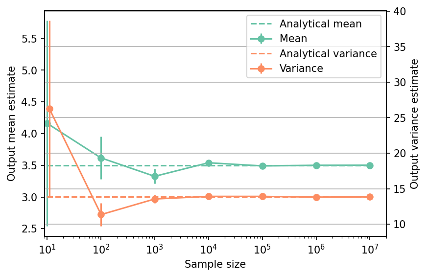
The tabulated results for each sample size is shown below.

from tabulate import tabulate

# --- Compile data row-wise
outputs = [
    [
        np.nan,
        mean_analytical,
        0.0,
        var_analytical,
        0.0,
        "Analytical",
    ]
]

for (
    sample_size,
    mean_estimate,
    mean_estimate_error,
    var_estimate,
    var_estimate_error,
) in zip(
    sample_sizes,
    mean_estimates,
    mean_estimates_errors,
    var_estimates,
    var_estimates_errors,
):
    outputs += [
        [
            sample_size,
            mean_estimate,
            mean_estimate_error,
            var_estimate,
            var_estimate_error,
            "Monte-Carlo",
        ],
    ]

header_names = [
    "Sample size",
    "Mean",
    "Mean error",
    "Variance",
    "Variance error",
    "Remark",
]

tabulate(
    outputs,
    headers=header_names,
    floatfmt=(".1e", ".4e", ".4e", ".4e", ".4e", "s"),
    tablefmt="html",
    stralign="center",
    numalign="center",
)

Sample size	Mean	Mean error	Variance	Variance error	Remark
nan	3.5000e+00	0.0000e+00	8.9169e+00	0.0000e+00	Analytical
1.0e+01	3.3079e+00	1.2312e+00	1.5159e+01	7.1458e+00	Monte-Carlo
1.0e+02	3.8445e+00	2.9416e-01	8.6529e+00	1.2299e+00	Monte-Carlo
1.0e+03	3.3626e+00	9.3054e-02	8.6591e+00	3.8744e-01	Monte-Carlo
1.0e+04	3.4921e+00	3.0054e-02	9.0327e+00	1.2775e-01	Monte-Carlo
1.0e+05	3.5048e+00	9.4424e-03	8.9160e+00	3.9874e-02	Monte-Carlo
1.0e+06	3.5032e+00	2.9860e-03	8.9164e+00	1.2610e-02	Monte-Carlo
1.0e+07	3.5007e+00	9.4437e-04	8.9184e+00	3.9884e-03	Monte-Carlo

Sensitivity indices#

The main-effect and total-effect Sobol’ indices of the Ishigami function can be
derived analytically.

The main-effect (i.e., first-order) Sobol’ indices are:

\(S_1 \equiv \frac{V_1}{\mathbb{V}[Y]}\)
\(S_2 \equiv \frac{V_2}{\mathbb{V}[Y]}\)
\(S_3 \equiv \frac{V_3}{\mathbb{V}[Y]}\)

where the total variances \(\mathbb{V}[Y]\) is given in the section above and
the partial variances are given by:

\(V_1 = \frac{1}{2} \, (1 + \frac{b \pi^4}{5})^2\)
\(V_2 = \frac{a^2}{8}\)
\(V_3 = 0\)

The total-effect Sobol’ indices, on the other hand:

\(ST_1 \equiv \frac{VT_1}{\mathbb{V}[Y]}\)
\(ST_2 \equiv \frac{VT_2}{\mathbb{V}[Y]}\)
\(ST_3 \equiv \frac{VT_3}{\mathbb{V}[Y]}\)

where:

\(VT_1 = \frac{1}{2} \, (1 + \frac{b \pi^4}{5})^2 + \frac{8 b^2 \pi^8}{225}\)
\(VT_2 = \frac{a^2}{8}\)
\(VT_3 = \frac{8 b^2 \pi^8}{225}\)

Note, once more, that the values of the partial variances depend on the parameter values.

Note

The Ishigami function has a peculiar dependence on \(X_3\); the main-effect index of the input variable is \(0\) but the total-effect index is not, due to an interaction with \(X_1\)!

Furthermore, as can be seen from the function definition, \(X_2\) has no interaction effect; its main-effect and total-effect indices are exactly the same.

References#

IH91(1,2,3): T. Ishigami and T. Homma. An importance quantification technique in uncertainty analysis for computer models. In [1990] Proceedings. First International Symposium on Uncertainty Modeling and Analysis, 398–403. IEEE Comput. Soc. Press, 1991. doi:10.1109/ISUMA.1990.151285.
SobolL99(1,2): Ilya M. Sobol' and Yu L. Levitan. On the use of variance reducing multipliers in Monte Carlo computations of a global sensitivity index. Computer Physics Communications, 117(1):52–61, 1999. doi:10.1016/S0010-4655(98)00156-8.
Sud08: Bruno Sudret. Global sensitivity analysis using polynomial chaos expansions. Reliability Engineering & System Safety, 93(7):964–979, 2008. doi:10.1016/j.ress.2007.04.002.
MILR09: Amandine Marrel, Bertrand Iooss, Béatrice Laurent, and Olivier Roustant. Calculations of Sobol indices for the Gaussian process metamodel. Reliability Engineering & System Safety, 94(3):742–751, 2009. doi:10.1016/j.ress.2008.07.008.

UQTestFuns

Ishigami Function

Contents