Flood Model#
import numpy as np
import matplotlib.pyplot as plt
import uqtestfuns as uqtf
The flood model is an eight-dimensional scalar valued function. The model was used in the context of sensitivity analysis in [IL15, LIPG13] and has become a canonical example of the OpenTURNS package [BDIP17].
Test function instance#
To create a default instance of the flood model:
my_testfun = uqtf.Flood()
Check if it has been correctly instantiated:
print(my_testfun)
Function ID      : Flood
Input Dimension  : 8 (fixed)
Output Dimension : 1
Parameterized    : False
Description      : Flood model from Iooss and Lemaître (2015)
Applications     : metamodeling, sensitivity
Description#
The flood model computes the maximum annual underflow of a river using the following analytical formula:
where \(\boldsymbol{x} = \{ q, k_s, z_v, z_m, h_d, c_b, l, b \}\) is the eight-dimensional vector of input variables further defined below. The output is given in \([\mathrm{m}]\). A negative value indicates that an overflow (flooding) occurs.
Note
Compared to the original function, this implementation inverted the sign of the output such that underflowing has a positive sign.
The model is based on a simplification of the one-dimensional hydro-dynamical equations of St. Venant under the assumption of uniform and constant flow rate and a large rectangular section.
Probabilistic input#
Based on [IL15] (Table 4), the probabilistic input model for the flood model consists of eight independent random variables with marginals shown in the table below.
Function ID     : Flood
Input ID        : Iooss2015
Input Dimension : 8
Description     : Probabilistic input model for the Flood model from Iooss
                  and Lemaître (2015)
Marginals       :

 No.    Name    Distribution          Parameters                     Description
-----  ------  --------------  -------------------------  ---------------------------------
  1      Q      trunc-gumbel   [1013.  558.  500. 3000.]  Maximum annual flow rate [m^3/s]
  2      Ks     trunc-normal       [30.  8. 15. inf]      Strickler coefficient [m^(1/3)/s]
  3      Zv      triangular          [49. 51. 50.]           River downstream level [m]
  4      Zm      triangular          [54. 56. 55.]            River upstream level [m]
  5      Hd       uniform               [7. 9.]                    Dyke height [m]
  6      Cb      triangular        [55.  56.  55.5]                Bank level [m]
  7      L       triangular       [4990. 5010. 5000.]      Length of the river stretch [m]
  8      B       triangular        [295. 305. 300.]                River width [m]

Copulas         : Independence
Reference results#
This section provides several reference results of typical UQ analyses involving the test function.
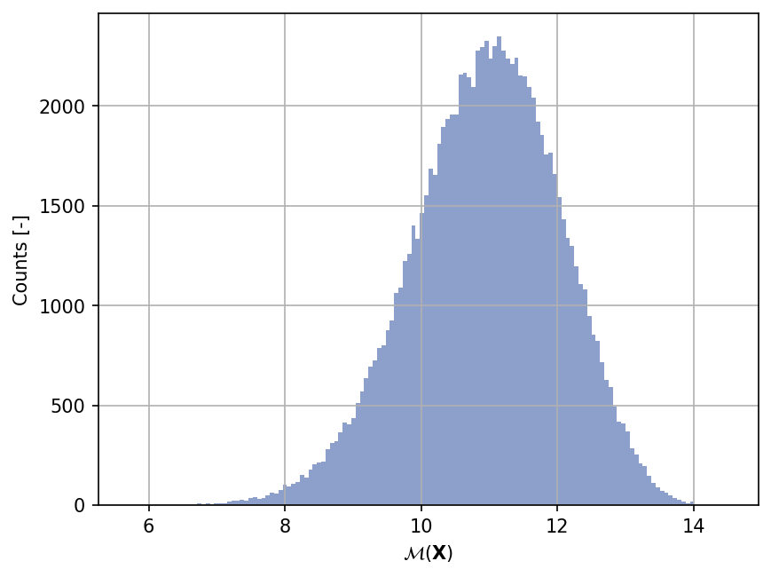
Sample histogram#
Shown below is the histogram of the output based on \(100'000\) random points:
Moments estimation#
Shown below is the convergence of a direct Monte-Carlo estimation of the output mean and variance with increasing sample sizes.
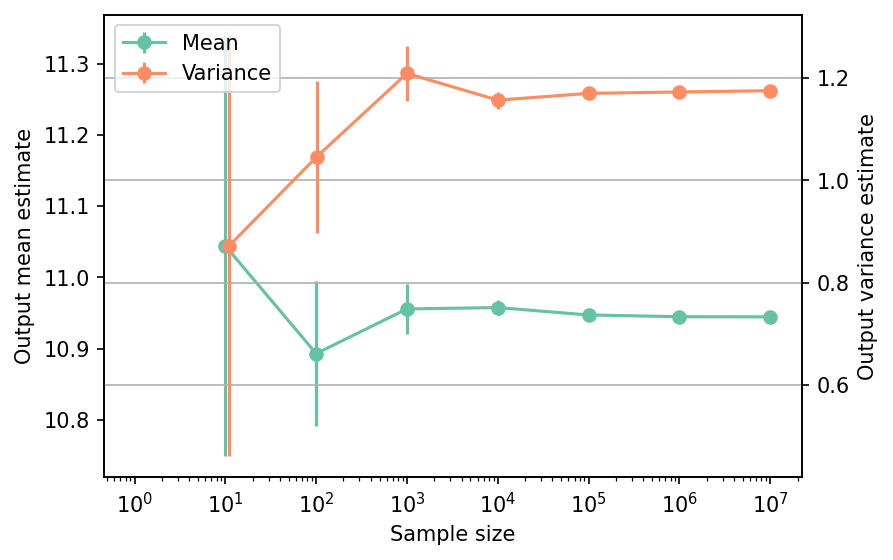
The tabulated results for each sample size is shown below.
| Sample size | Mean | Mean error | Variance | Variance error | Remark |
|---|---|---|---|---|---|
| 10 | 1.1044e+01 | 2.9528e-01 | 8.7189e-01 | 4.1101e-01 | Monte-Carlo |
| 100 | 1.0893e+01 | 1.0227e-01 | 1.0459e+00 | 1.4866e-01 | Monte-Carlo |
| 1000 | 1.0956e+01 | 3.4778e-02 | 1.2095e+00 | 5.4119e-02 | Monte-Carlo |
| 10000 | 1.0958e+01 | 1.0757e-02 | 1.1571e+00 | 1.6365e-02 | Monte-Carlo |
| 100000 | 1.0947e+01 | 3.4212e-03 | 1.1704e+00 | 5.2344e-03 | Monte-Carlo |
| 1000000 | 1.0945e+01 | 1.0831e-03 | 1.1731e+00 | 1.6591e-03 | Monte-Carlo |
| 10000000 | 1.0945e+01 | 3.4287e-04 | 1.1756e+00 | 5.2574e-04 | Monte-Carlo |
References#
Bertrand Iooss and Paul Lemaître. A review on global sensitivity analysis methods. In Uncertainty Management in Simulation-Optimization of Complex Systems, pages 101–122. Springer US, 2015. doi:10.1007/978-1-4899-7547-8_5.
Michaël Baudin, Anne Dutfoy, Bertrand Iooss, and Anne-Laure Popelin. OpenTURNS: an industrial software for uncertainty quantification in simulation. In Handbook of Uncertainty Quantification, pages 2001–2038. Springer International Publishing, 2017. doi:10.1007/978-3-319-12385-1_64.
M. Lamboni, B. Iooss, A.-L. Popelin, and F. Gamboa. Derivative-based global sensitivity measures: General links with Sobol' indices and numerical tests. Mathematics and Computers in Simulation, 87:45–54, 2013. doi:10.1016/j.matcom.2013.02.002.