Oakley and O’Hagan (2002) One-dimensional (1D) Function#

The 1D function from Oakley and O’Hagan (2002) (or Oakley1D function for short) is a scalar-valued test function. It was used in [OOHagan02] as a test function for illustrating metamodeling and uncertainty propagation approaches.

import numpy as np
import matplotlib.pyplot as plt
import uqtestfuns as uqtf

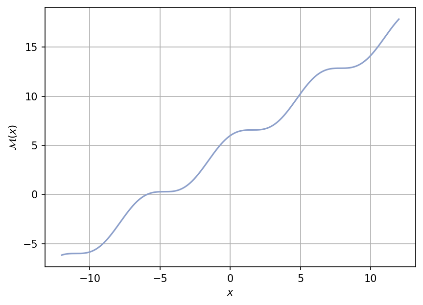
A plot of the function is shown below for \(x \in [-12, 12]\).

Test function instance#

To create a default instance of the test function:

my_testfun = uqtf.Oakley1D()

Check if it has been correctly instantiated:

print(my_testfun)

Name              : Oakley1D
Spatial dimension : 1
Description       : One-dimensional function from Oakley and O'Hagan (2002)

Description#

The test function is analytically defined as follows:

\[ \mathcal{M}(x) = 5 + x + \cos{x}, \]

where \(x\) is probabilistically defined below.

Probabilistic input#

Based on [OOHagan02], the probabilistic input model for the 1D Oakley-O’Hagan function consists of a normal random variable with the parameters shown in the table below.

my_testfun.prob_input

Name: Oakley2002

Spatial Dimension: 1

Description: Probabilistic input model for the one-dimensional function from Oakley and O'Hagan (2002)

Marginals:

No.	Name	Distribution	Parameters	Description
1	x	normal	[0. 4.]	None

Copulas: None

Reference results#

This section provides several reference results of typical UQ analyses involving the test function.

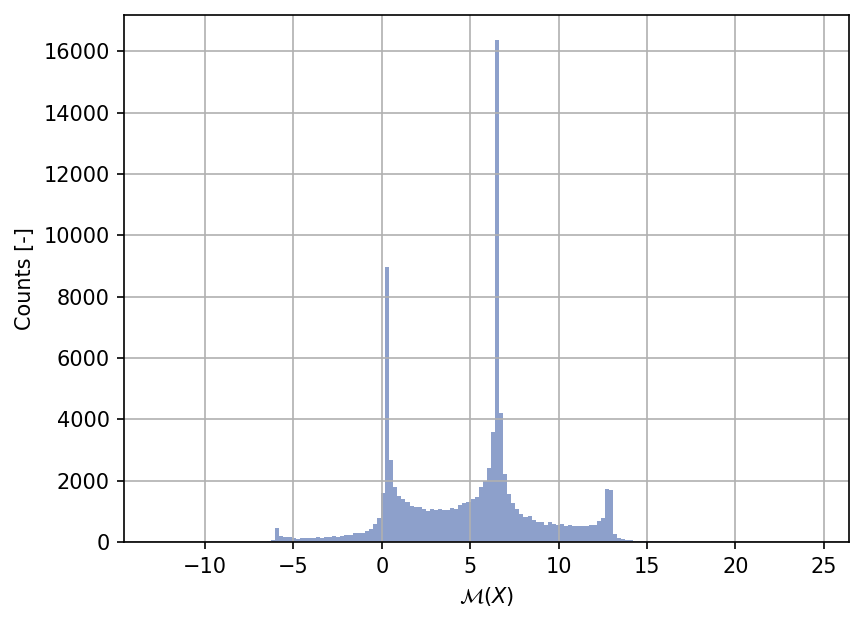
Sample histogram#

Shown below is the histogram of the output based on \(100'000\) random points:

np.random.seed(42)
xx_test = my_testfun.prob_input.get_sample(100000)
yy_test = my_testfun(xx_test)

plt.hist(yy_test, bins="auto", color="#8da0cb");
plt.grid();
plt.ylabel("Counts [-]");
plt.xlabel("$\mathcal{M}(X)$");
plt.gcf().tight_layout(pad=3.0)
plt.gcf().set_dpi(150);

Moment estimations#

Shown below is the convergence of a direct Monte-Carlo estimation of the output mean and variance with increasing sample sizes.

np.random.seed(42)
sample_sizes = np.array([1e1, 1e2, 1e3, 1e4, 1e5, 1e6], dtype=int)
mean_estimates = np.empty((len(sample_sizes), 50))
var_estimates = np.empty((len(sample_sizes), 50))

for i, sample_size in enumerate(sample_sizes):
    for j in range(50):
        xx_test = my_testfun.prob_input.get_sample(sample_size)
        yy_test = my_testfun(xx_test)
        mean_estimates[i, j] = np.mean(yy_test)
        var_estimates[i, j] = np.var(yy_test)

# --- Compute the error associated with the estimates
mean_estimates_errors = np.std(mean_estimates, axis=1)
var_estimates_errors = np.std(var_estimates, axis=1)

# --- Plot the mean and variance estimates
fig, ax_1 = plt.subplots(figsize=(6,4))

# --- Mean plot
ax_1.errorbar(
    sample_sizes,
    mean_estimates[:,0],
    yerr=2.0*mean_estimates_errors,
    marker="o",
    color="#66c2a5",
    label="Mean"
)
ax_1.set_xlim([5, 2e6])
ax_1.set_xlabel("Sample size")
ax_1.set_ylabel("Output mean estimate")
ax_1.set_xscale("log");
ax_2 = ax_1.twinx()

# --- Variance plot
ax_2.errorbar(
    sample_sizes+1,
    var_estimates[:,0],
    yerr=1.96*var_estimates_errors,
    marker="o",
    color="#fc8d62",
    label="Variance",
)
ax_2.set_ylabel("Output variance estimate")

# Add the two plots together to have a common legend
ln_1, labels_1 = ax_1.get_legend_handles_labels()
ln_2, labels_2 = ax_2.get_legend_handles_labels()
ax_2.legend(ln_1 + ln_2, labels_1 + labels_2, loc=0)

plt.grid()
fig.set_dpi(150)

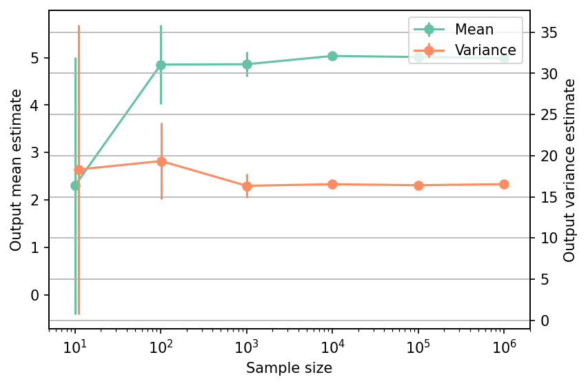
The tabulated results for each sample size is shown below.

from tabulate import tabulate

# --- Compile data row-wise
outputs =[]

for (
    sample_size,
    mean_estimate,
    mean_estimate_error,
    var_estimate,
    var_estimate_error,
) in zip(
    sample_sizes,
    mean_estimates[:,0],
    2.0*mean_estimates_errors,
    var_estimates[:,0],
    2.0*var_estimates_errors,
):
    outputs += [
        [
            sample_size,
            mean_estimate,
            mean_estimate_error,
            var_estimate,
            var_estimate_error,
            "Monte-Carlo",
        ],
    ]

header_names = [
    "Sample size",
    "Mean",
    "Mean error",
    "Variance",
    "Variance error",
    "Remark",
]

tabulate(
    outputs,
    numalign="center",
    stralign="center",
    tablefmt="html",
    floatfmt=(".1e", ".4e", ".4e", ".4e", ".4e", "s"),
    headers=header_names
)

Sample size	Mean	Mean error	Variance	Variance error	Remark
1.0e+01	5.3667e+00	2.5821e+00	1.2412e+01	1.4007e+01	Monte-Carlo
1.0e+02	5.0586e+00	7.4662e-01	1.3622e+01	4.0659e+00	Monte-Carlo
1.0e+03	5.1161e+00	2.2424e-01	1.6265e+01	1.1872e+00	Monte-Carlo
1.0e+04	4.9933e+00	8.0880e-02	1.6864e+01	5.4213e-01	Monte-Carlo
1.0e+05	4.9998e+00	2.5349e-02	1.6542e+01	1.3712e-01	Monte-Carlo
1.0e+06	4.9988e+00	7.3062e-03	1.6518e+01	4.4011e-02	Monte-Carlo

References#

OOHagan02(1,2): Jeremy Oakley and Anthony O'Hagan. Bayesian inference for the uncertainty distribution of computer model outputs. Biometrika, 89(4):769–784, 2002. doi:10.1093/biomet/89.4.769.

UQTestFuns

Oakley and O’Hagan (2002) One-dimensional (1D) Function

Contents