Hyper-sphere Bound

import numpy as np
import matplotlib.pyplot as plt
import uqtestfuns as uqtf

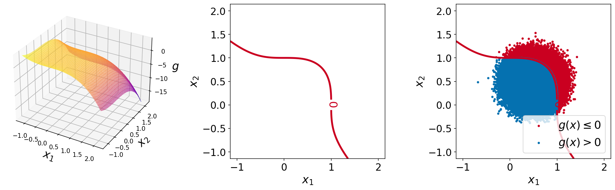
The hyper-sphere bound problem is a two-dimensional function used in [LGG+18] as a test function for reliability analysis algorithms.

The plots of the function are shown below. The left plot shows the surface plot of the performance function, the center plot shows the contour plot with a single contour line at function value of \(0.0\) (the limit-state surface), and the right plot shows the same plot with \(10^6\) sample points overlaid.

Test function instance

To create a default instance of the test function:

my_testfun = uqtf.HyperSphere()

Check if it has been correctly instantiated:

print(my_testfun)

Name              : HyperSphere
Spatial dimension : 2
Description       : Hyper-sphere bound reliability problem from Li et al. (2018)

Description

The test function (i.e., the performance function) is analytically defined as follows 1:

\[ g(\boldsymbol{x}) = 1 - x_1^3 - x_2^3 \]

where \(\boldsymbol{x} = \{ x_1, x_2 \}\) is the two-dimensional vector of input variables probabilistically defined further below.

The failure state and the failure probability are defined as \(g(\boldsymbol{x}) \leq 0\) and \(\mathbb{P}[g(\boldsymbol{X}) \leq 0]\), respectively.

Probabilistic input

Based on [LGG+18], the probabilistic input model for the test function consists of two independent standard normal random variables (see the table below).

my_testfun.prob_input

Name: Li2018

Spatial Dimension: 2

Description: Input model for the hyper-sphere reliability problem from Li et al. (2018)

Marginals:

No.	Name	Distribution	Parameters	Description
1	X1	normal	[0.5 0.2]	None
2	X2	normal	[0.5 0.2]	None

Copulas: None

Reference results

This section provides several reference results of typical UQ analyses involving the test function.

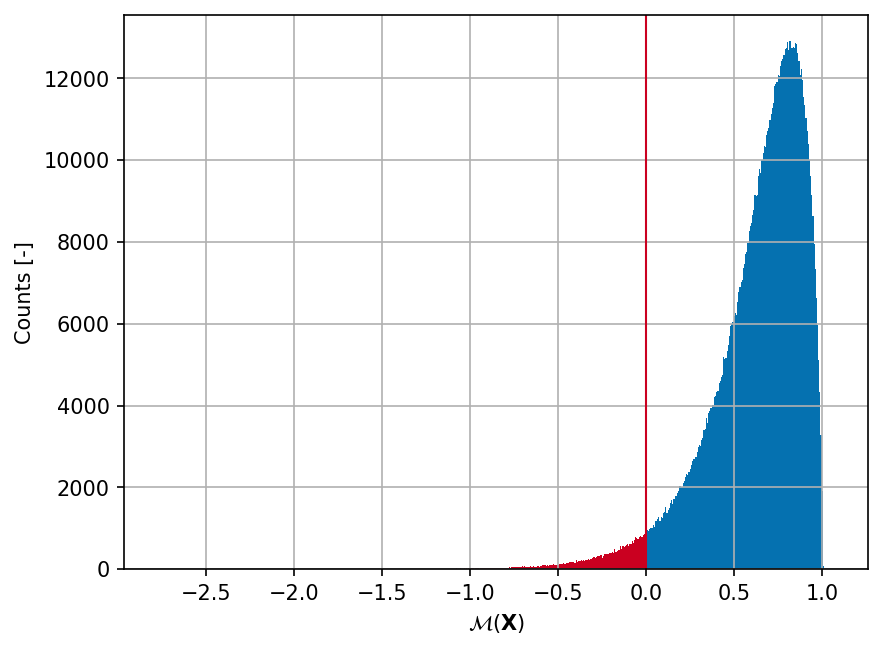
Sample histogram

Shown below is the histogram of the output based on \(10^6\) random points:

xx_test = my_testfun.prob_input.get_sample(1000000)
yy_test = my_testfun(xx_test)
idx_pos = yy_test > 0
idx_neg = yy_test <= 0

hist_pos = plt.hist(yy_test, bins="auto", color="#0571b0")
plt.hist(yy_test[idx_neg], bins=hist_pos[1], color="#ca0020")
plt.axvline(0, linewidth=1.0, color="#ca0020")

plt.grid()
plt.ylabel("Counts [-]")
plt.xlabel("$\mathcal{M}(\mathbf{X})$")
plt.gcf().set_dpi(150);

Failure probability (\(P_f\))

Some reference values for the failure probability \(P_f\) from the literature are summarized in the table below.

Method	\(N\)	\(\hat{P}_f\)	\(\mathrm{CoV}[\hat{P}_f]\)	Source
MCS	\(10^6\)	\(3.381 \times 10^{-2}\)	—2	[LGG+18]
FORM	\(15\)	\(1.891 \times 10^{-2}\)	—	[LGG+18]
SORM	\(20\)	\(2.672 \times 10^{-2}\)	—	[LGG+18]
SSRM	\(12\)	\(3.381 \times 10^{-2}\)	—2	[LGG+18]

References

LGG+18(1,2,3,4,5,6,7,8)

Xu Li, Chunlin Gong, Liangxian Gu, Wenkun Gao, Zhao Jing, and Hua Su. A sequential surrogate method for reliability analysis based on radial basis function. Structural Safety, 73:42–53, 2018. doi:10.1016/j.strusafe.2018.02.005.

---

1

see Eq. (10) in [LGG+18].

2(1,2)

The coefficient of variations of the failure probability estimates in [LGG+18] were not reported.