Tutorial: Test a Sensitivity Analysis Method#
UQTestFuns includes a wide range of test functions from the literature employed in a sensitivity analysis exercise. In this tutorial, you’ll implement a sensitivity analysis method and test the implemented method using a test function available in UQTestFuns (the popular Ishigami function). Afterward, you’ll compare the results against analytical results.
By the end of this tutorial, you’ll get an idea how a function from UQTestFuns is used to test a sensitivity analysis method.
import numpy as np
import matplotlib.pyplot as plt
import uqtestfuns as uqtf
Global sensitivity analysis#
Sensitivity analysis is a model inference technique whose overarching goal is to understand the inputs/outputs relationship of a complex (potentially, black box) model. Specific goals include:
identification of inputs that drive output variability that leads to factor prioritization, that is, identifying which inputs that result in the largest reduction in the output variability.
identification of non-influential inputs that leads to factor fixing, that is, identifying which inputs that can be fixed at any value without affecting the output.
A global sensitivity analysis is often distinguished from a local analysis. A local analysis is concerned with the effects of perturbation around a particular instance of the inputs (e.g., their nominal values) on the output. A global analysis, on the other hand, is concerned with the effects of variations over all possible instances of inputs within their respective uncertainty range on the output.
Variance decomposition#
Consider an \(M\)-dimensional mathematical function \(\mathcal{M}: \mathcal{D}_{\boldsymbol{X}} \in [0, 1]^M \mapsto \mathbb{R}\) that represents a computational model of interest.
Due to uncertain inputs, represented as an \(M\)-dimensional random vector \(\boldsymbol{X}\), the output of the model becomes a random variable \(Y = \mathcal{M}(\boldsymbol{X})\). It is further assumed that the components \(X_m\)’s of the random vector \(\boldsymbol{X}\) are mutually independent such that the joint probability density function \(f_{\boldsymbol{X}}\) reads:
where \(f_{X_m}\) is the marginal probability density function of \(X_m\).
The Hoeffding-Sobol’ variance decomposition of random variable \(Y\) reads as follows:
where the terms are partial variances defined below:
\(V_m = \mathbb{V}_{X_m} \left[ \mathbb{E}_{X_{\sim m}}\left[ Y | X_m \right]\right]\)
\(V_{m, n} = \mathbb{V}_{X_{\{m, n\}}} \left[ \mathbb{E}_{X_{\sim \{m, n\}}}\left[ Y | X_m, X_n \right]\right]\)
etc.
Sobol’ sensitivity indices#
By normalizing the above equation with the total variance \(\mathbb{V}[Y]\), we obtain the following expression:
where now each term is a normalized partial variance. These normalized terms are called Sobol’ sensitivity indices and there are \(2^M - 1\) (where \(M\) is the number of dimension) indices.
Of particular importance is the first-order (or main-effect) Sobol’ index \(S_m\) defined as follows [Sobol93]:
This index indicates the importance of a particular input variable on the output variance. These indices are aligned with the aforementioned factor prioritization goal of sensitivity analysis.
Another sensitivity index of particular importance is the total-effect Sobol’ index defined for input variable \(m\) below [HS96]:
Monte-Carlo estimation#
Warning
A method to estimate the main-effect and total-effect indices via a Monte-Carlo simulation is implemented here following the most naive and straightforward approach. It is only to serve as an illustration. This implementation is, however, not the state-of-the-art approach to estimate the indices (see, for instance, [Sal02, SAA+10]). Please refer to a dedicated sensitivity analysis and uncertainty quantification package for a proper analysis.
The estimation of the Sobol’ sensitivity indices as defined in the above equations can be directly carried out using a Monte-Carlo simulation. The most straightforward, though rather naive and computationally expensive, method is to use a nested loop for the computation of the conditional variances and expectations appearing in both indices.
For instance, in the estimation of the first-order index of, say, input variable \(x_m\), the outer loop samples values of \(X_m\) while the inner loop samples values of \(\boldsymbol{X}_{\sim m}\) (i.e., all input variables except \(x_m\)). The cost of the analysis in terms of the model evaluations for estimating the first-order index for each input variable is \(N^2\) where \(N\) is the Monte-Carlo sample size. It is expected that size of \(N\) is between \(10^3\) and \(10^6\).
Algorithm 1 below illustrates the procedure to compute main-effect Sobol’ indices.
Algorithm 1 (Brute force MC for estimating all \(S_m\))
Inputs A computational model \(\mathcal{M}\), random input variables \(\boldsymbol{X} = \{ X_1, \ldots, X_M \}\), number of MC sample points \(N\)
Output First-order Sobol’ sensitivity indices \(S_m\) for \(m = 1, \ldots, M\)
For \(m = 1\) to \(M\):
\(\Sigma_i \leftarrow 0\)
\(\Sigma_i^2 \leftarrow 0\)
For \(i = 1\) to \(N\):
Sample \(x_m^{(i)}\) from \(X_m\)
\(\Sigma_j \leftarrow 0\)
For \(j = 1\) to \(N\):
Sample \(\boldsymbol{x}_{\sim m}^{(j)}\) from \(\boldsymbol{X}_{\sim m}\)
\(\Sigma_j \leftarrow \Sigma_j + \mathcal{M}(x_m^{(j)}, \boldsymbol{x}_{\sim m}^{(j)})\)
\(\mathbb{E}_{\boldsymbol{X}_{\sim m}}\left[ Y | X_m \right]^{(i)} \leftarrow \frac{1}{N} \Sigma_j\)
\(\Sigma_i \leftarrow \Sigma_i + \mathbb{E}_{\boldsymbol{X}_{\sim m}}\left[ Y | X_m \right]^{(i)}\)
\(\Sigma_{i^2} \leftarrow \Sigma_{i^2} + \left( \mathbb{E}_{\boldsymbol{X}_{\sim m}}\left[ Y | X_m \right]^{(i)} \right)^2\)
\(\mathbb{V}_{X_m} \left[ \mathbb{E}_{\boldsymbol{X}_{\sim m}}\left[ Y | X_m \right]\right] \leftarrow \frac{1}{N} \Sigma_{i^2} - \left( \frac{1}{N} \Sigma_{i} \right)^2\)
\(S_m \leftarrow \frac{\mathbb{V}_{X_m} \left[ \mathbb{E}_{\boldsymbol{X}_{\sim m}}\left[ Y | X_m \right]\right]}{\mathbb{V}[Y]}\)
The output variance \(\mathbb{V}[Y]\) used in the above algorithm can be computed following Algorithm 2.
Algorithm 2 (Brute force MC for estimating output variance \(\mathbb{V}[Y]\))
Inputs A computational model \(\mathcal{M}\), random input variables \(\boldsymbol{X}\), number of MC sample points \(N\)
Output Output variance \(\mathbb{V}[Y]\)
\(\Sigma_i \leftarrow 0\)
\(\Sigma_i^2 \leftarrow 0\)
For \(i = 1\) to \(N\):
Sample \(\boldsymbol{x}^{(i)}\) from \(\boldsymbol{X}\)
\(\Sigma_i \leftarrow \Sigma_i + \mathcal{M}(\boldsymbol{x}^{(i)})\)
\(\Sigma_{i^2} \leftarrow \Sigma_{i^2} + \left( \mathcal{M}(\boldsymbol{x}^{(i)} \right)^2\)
\(\mathbb{V}[Y] \leftarrow \frac{1}{N} \Sigma_{i^2} - \left( \frac{1}{N} \Sigma_i \right)^2\)
Similar Monte-Carlo algorithm can be devised to compute the total-effect Sobol’ indices as shown in Algorithm 3.
Algorithm 3 (Brute force MC for estimating all \(ST_m\))
Inputs A computational model \(\mathcal{M}\), random input variables \(\boldsymbol{X} = \{ X_1, \ldots, X_M \}\), number of MC sample points \(N\)
Output First-order Sobol’ sensitivity indices \(S_m\) for \(m = 1, \ldots, M\)
For \(m = 1\) to \(M\):
\(\Sigma_i \leftarrow 0\)
\(\Sigma_i^2 \leftarrow 0\)
For \(i = 1\) to \(N\):
Sample \(\boldsymbol{x}_{\sim m}^{(i)}\) from \(\boldsymbol{X}_{\sim m}\)
\(\Sigma_j \leftarrow 0\)
For \(j = 1\) to \(N\):
Sample \(x_{m}^{(j)}\) from \(X_m\)
\(\Sigma_j \leftarrow \Sigma_j + \mathcal{M}(x_m^{(j)}, \boldsymbol{x}_{\sim m}^{(j)})\)
\(\mathbb{E}_{X_m}\left[ Y | \boldsymbol{X}_{\sim m} \right]^{(i)} \leftarrow \frac{1}{N} \Sigma_j\)
\(\Sigma_i \leftarrow \Sigma_i + \mathbb{E}_{X_m}\left[ Y | \boldsymbol{X}_{\sim m} \right]^{(i)}\)
\(\Sigma_{i^2} \leftarrow \Sigma_{i^2} + \left( \mathbb{E}_{X_m}\left[ Y | \boldsymbol{X}_{\sim m} \right]^{(i)} \right)^2\)
\(\mathbb{V}_{\boldsymbol{X}_{\sim m}} \left[ \mathbb{E}_{X_m}\left[ Y | \boldsymbol{X}_{\sim m} \right]\right] \leftarrow \frac{1}{N} \Sigma_{i^2} - \left( \frac{1}{N} \Sigma_{i} \right)^2\)
\(ST_m \leftarrow 1 - \frac{\mathbb{V}_{\boldsymbol{X}_{\sim m}} \left[ \mathbb{E}_{X_m}\left[ Y | \boldsymbol{X}_{\sim m} \right]\right]}{\mathbb{V}[Y]}\)
These algorithms are implemented in a Python function that returns the main-effect and total-effect Sobol’ indices of all the input variables of a computational model. The function assumes that a probabilistic input model of the computational model has been defined such that sample points may be generated from them.
Note
And indeed, test functions included in UQTestFuns are all given with the corresponding probabilistic input model according to the literature.
Ishigami function#
To test the implemented algorithm above, we choose the popular Ishigami function [IH91] whose analytical values for the sensitivity indices are known. The function is highly non-linear and non-monotonous and given as follows:
where \(\boldsymbol{x} = \{ x_1, x_2, x_3 \}\) is the three-dimensional vector of input variables further defined in the table below, and \(a\) and \(b\) are parameters of the function.
To create an instance of the Ishigami function:
ishigami = uqtf.Ishigami()
The input variables of the function are probabilistically defined according to the table below.
print(ishigami.prob_input)
Function ID     : Ishigami
Input ID        : Ishigami1991
Input Dimension : 3
Description     : Probabilistic input model for the Ishigami function from
                  Ishigami and Homma (1991).
Marginals       :

 No.    Name    Distribution          Parameters           Description
-----  ------  --------------  -------------------------  -------------
  1      X1       uniform      [-3.14159265  3.14159265]        -
  2      X2       uniform      [-3.14159265  3.14159265]        -
  3      X3       uniform      [-3.14159265  3.14159265]        -

Copulas         : Independence
Finally, the default values for the parameters \(a\) and \(b\) are:
print(ishigami.parameters)
Function ID  : Ishigami
Parameter ID : Ishigami1991
Description  : Parameter set for the Ishigami function from Ishigami and
               Homma (1991)

 No.    Keyword      Value      Type    Description
-----  ---------  -----------  ------  -------------
  1        a      7.00000e+00  float
  2        b      1.00000e-01  float
For reproducibility of this tutorial, set the seed number for the pseudo-random generator attached to the probabilistic input model:
ishigami.prob_input.reset_rng(452397)
The variance of the Ishigami function can be analytically derived and it is a function of the parameters:
The analytical sensitivity indices are also available as shown in the table below also as functions of the parameters.
Input variable |
\(S_m\) |
\(ST_m\) |
|---|---|---|
\(1\) |
\(\frac{1}{\mathbb{V}[Y]} \frac{1}{2} (1 + \frac{b \pi^4}{5})^2\) |
\(\frac{1}{\mathbb{V}[Y]} \left( \frac{1}{2} \, (1 + \frac{b \pi^4}{5})^2 + \frac{8 b^2 \pi^8}{225} \right)\) |
\(2\) |
\(\frac{1}{\mathbb{V}[Y]} \frac{a^2}{8}\) |
\(\frac{a^2}{8 \mathbb{V}[Y]}\) |
\(3\) |
\(0.0\) |
\(\frac{8 b^2 \pi^8}{225 \mathbb{V}[Y]}\) |
Notice that while \(X_3\) does not directly influence the output variance by itself (it’s main-effect index is zero), it does influence the output variance via interaction with \(X_1\). Furthermore, \(X_2\) has no interaction effect whatsoever as its main-effect and total-effect indices are the same.
For later comparison, we define a Python function that returns the analytical values of the Sobol’ indices of the Ishigami function.
Sobol’ indices estimation#
To observe the convergence of the estimation procedure implemented above, several Monte-Carlo sample sizes are used:
sample_sizes = np.arange(0, 3500, 500)[1:]
first_order_indices = np.zeros((len(sample_sizes), ishigami.input_dimension))
total_effect_indices = np.zeros((len(sample_sizes), ishigami.input_dimension))

for i, sample_size in enumerate(sample_sizes):
  first_order_indices[i, :], total_effect_indices[i, :] = estimate_sobol_indices(
      ishigami, ishigami.prob_input, sample_size
  )
Compute the analytical values for the given parameters:
first_order_ref, total_effect_ref = compute_sobol_indices(**ishigami.parameters.as_dict())
The estimated indices as a function of sample size is plotted below; the estimated values are in solid lines while the analytical values are in dashed lines.
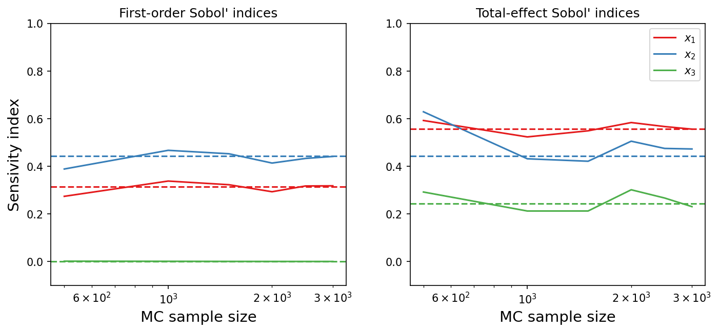
The implemented method seems to estimate the indices relatively well; increasing the Monte-Carlo sample size would improve the accuracy of the estimates but with a high computational cost.
The challenge for a sensitivity analysis method is to ascertain the importance (or non-importance) of input variables either qualitatively or quantitatively with as few computational model evaluations as possible.
References#
T. Ishigami and T. Homma. An importance quantification technique in uncertainty analysis for computer models. In [1990] Proceedings. First International Symposium on Uncertainty Modeling and Analysis, 398–403. IEEE Comput. Soc. Press, 1991. doi:10.1109/ISUMA.1990.151285.
Ilya M. Sobol'. Sensitivity estimates for nonlinear mathematical models. Mathematical Modelling and Computational Experiments, 1(4):407–414, 1993.
Toshimitsu Homma and Andrea Saltelli. Importance measures in global sensitivity analysis of nonlinear models10.1007/978-3-319-11259-6_24-1. Reliability Engineering & System Safety, 52(1):1–17, 1996. doi:10.1016/0951-8320(96)00002-6.
Andrea Saltelli. Making best use of model evaluations to compute sensitivity indices. Computer Physics Communications, 145(2):280–297, 2002. doi:10.1016/s0010-4655(02)00280-1.
Andrea Saltelli, Paola Annoni, Ivano Azzini, Francesca Campolongo, Marco Ratto, and Stefano Tarantola. Variance based sensitivity analysis of model output. design and estimator for the total sensitivity index. Computer Physics Communications, 181(2):259–270, 2010. doi:10.1016/j.cpc.2009.09.018.