Beta Distribution

The Beta distribution is a four-parameter continuous probability distribution. The table below summarizes some important aspects of the distribution.

Notation	\(X \sim \mathrm{Beta}(\alpha, \beta, a, b)\)
Parameters	\(\alpha > 0\) (1st shape parameter)
	\(\beta > 0\) (2nd shape parameter)
	\(a \in (-\infty, b)\) (lower bound)
	\(b \in (a, \infty)\) (upper bound)
Support	\(\mathcal{D}_X = (0, 1)\)
PDF	\(f_X (x; \alpha, \beta, a, b) = \begin{cases} \frac{(x-a)^{\alpha-1} (b-x)^{\beta-1}}{(b-a)^{\alpha+\beta-1} B(\alpha, \beta)} & x \in [a, b] \\ 0 & x \notin [a, b] \end{cases}\)
CDF	\(F_X (x; \alpha, \beta, a, b) = \begin{cases} 0 & x < a \\ \frac{1}{(b-a)^{\alpha+\beta-1} B(\alpha,\beta)} B(x; \alpha, \beta, a, b) & x \in [a, b] \\ 1 & x > b \end{cases}\)
ICDF	\(F^{-1}_X (x; \alpha, \beta, a, b) = \left\{ y \, \vert \, \frac{B(y; \alpha, \beta, a, b)}{(b - a)^{\alpha + \beta - 1} B(\alpha, \beta)} = x \right\}\)

Beta function and incomplete Beta function

In the table above, \(B(\alpha, \beta)\) and \(B(x; \alpha, \beta, a, b)\) correspond to the Beta function and incomplete beta function on \((a, b)\), respectively. The Beta function is defined as

\[ B(\alpha, \beta) \equiv \int_0^1 t^{\alpha-1} (1 - t)^{\beta-1} dt = \frac{\Gamma(\alpha) \Gamma(\beta)}{\Gamma(\alpha + \beta)} \]

where \(\Gamma\) is the the Gamma function for positive real numbers

\[ \Gamma(x) = \int_0^\infty t^{x - 1} e^{-t} dt, \; x > 0. \]

The incomplete Beta function is defined as

\[ B(x; \alpha, \beta, a, b) \equiv \int_a^x (t - a)^{\alpha - 1} (b - t)^{\beta - 1} dt. \]

Note the difference between the above formulation with the usual incomplete Beta function defined on \((0, 1)\):

\[ B(x; \alpha, \beta) \equiv \int_0^x t^{\alpha - 1} (1 - t)^{\beta - 1} dt \]

Note

The inverse cumulative distribution function (ICDF) of the Beta distribution is given as an implicit equation and must be solved numerically.

The plots of probability density functions (PDFs), sample histogram (of \(5'000\) points), cumulative distribution functions (CDFs), and inverse cumulative distribution functions (ICDFs) for different parameter values are shown below.

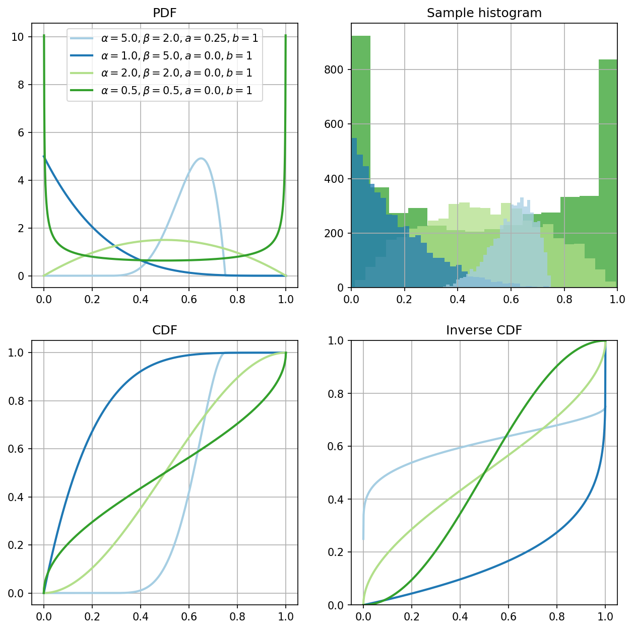
As can be observed from the plots above, that:

• if \(\alpha > 1.0\) and \(\beta > 1.0\), then the density is unimodal;

• if \(\alpha \leq 1.0\) or \(\beta \leq 1.0\), then the density is peaked at one or both boundaries;

• if \(\alpha = \beta\), then the density function is symmetrical.

Note that when \(\alpha = 1.0\) and \(\beta = 1.0\), then the density is a uniform density on \([0, 1]\); this is a special case of the Beta distribution.