Circular Pipe Crack#
import numpy as np
import matplotlib.pyplot as plt
import uqtestfuns as uqtf
The two-dimensional circular pipe crack reliability problem was introduced in [VAK15] and used, for instance, in [LGG+18].
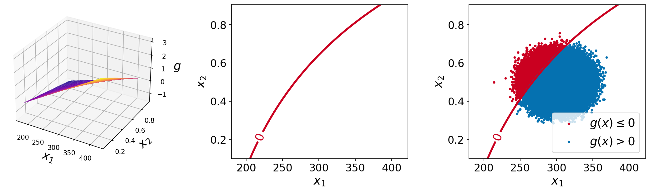
The plots of the function are shown below. The left plot shows the surface plot of the performance function, the center plot shows the contour plot with a single contour line at function value of \(0.0\) (the limit-state surface), and the right plot shows the same plot with \(10^6\) sample points overlaid.
Test function instance#
To create a default instance of the test function:
my_testfun = uqtf.CircularPipeCrack()
Check if it has been correctly instantiated:
print(my_testfun)
Function ID      : CircularPipeCrack
Input Dimension  : 2 (fixed)
Output Dimension : 1
Parameterized    : True
Description      : Circular pipe under bending moment from Verma et al. (2015)
Applications     : reliability
Description#
The system under consideration is as a circular pipe with a circumferential through-wall crack under a bending moment. The performance function is analytically defined as follows[1]:
where \(\boldsymbol{x} = \{ \sigma_f, \theta \}\) is the two-dimensional vector of input variables probabilistically defined further below; and \(\boldsymbol{p} = \{ t, R, M \}\) is the vector of deterministic parameters.
The failure state and the failure probability are defined as \(g(\boldsymbol{x}; \boldsymbol{p}) \leq 0\) and \(\mathbb{P}[g(\boldsymbol{X}; \boldsymbol{p}) \leq 0]\), respectively.
Probabilistic input#
Based on [VAK15], the probabilistic input model for the test function consists of two independent standard normal random variables (see the table below).
Function ID     : CircularPipeCrack
Input ID        : Verma2015
Input Dimension : 2
Description     : Input model for the circular pipe crack problem from
                  Verma et al. (2015)
Marginals       :

 No.    Name     Distribution      Parameters          Description
-----  -------  --------------  -----------------  --------------------
  1    sigma_f      normal      [301.079  14.78 ]   flow stress [MNm]
  2     theta       normal        [0.503 0.049]    half crack angle [-]

Copulas         : Independence
Parameters#
From [VAK15], the values of the parameters are as follows:
Parameter |
Value |
Description |
|---|---|---|
\(t\) |
\(3.377 \times 10^{-1}\) |
Radius of the pipe \([\mathrm{m}]\) |
\(R\) |
\(3.377 \times 10^{-2}\) |
Thickness of the pipe \([\mathrm{m}]\) |
\(M\) |
\(3.0\) |
Applied bending moment \([\mathrm{MNm}]\) |
Reference results#
This section provides several reference results of typical UQ analyses involving the test function.
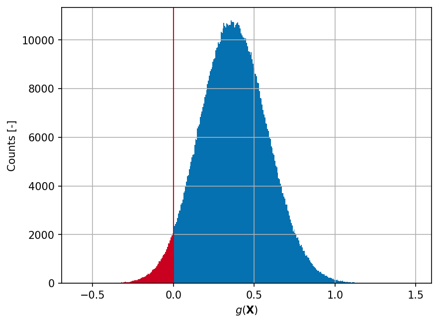
Sample histogram#
Shown below is the histogram of the output based on \(10^6\) random points:
Failure probability (\(P_f\))#
Some reference values for the failure probability \(P_f\) from the literature are summarized in the table below.