Tutorial: Create Built-in Test Functions#
UQTestFuns includes a wide range of test functions from the uncertainty quantification community; these functions are referred to as the built-in test functions. This tutorial provides you with an overview of the package; you’ll learn about the built-in test functions, their common interfaces, as well as their important properties and methods.
By the end of this tutorial, you’ll be able to create any test function available in UQTestFuns and access its basic but important functionalities.
UQTestFuns is designed to work with minimal dependency within the numerical Python ecosystem. At the very least, UQTestFuns requires NumPy and SciPy to work. It might be a good idea to import NumPy alongside UQTestFuns:
import numpy as np
import uqtestfuns as uqtf
Listing available test functions#
To list all the test functions currently available:
uqtf.list_functions()
+-------+-------------------------------+-----------+------------+----------+---------------+--------------------------------+
| No. | Constructor | # Input | # Output | Param. | Application | Description |
+=======+===============================+===========+============+==========+===============+================================+
| 1 | Ackley() | M | 1 | True | optimization, | Optimization test function |
| | | | | | metamodeling | from Ackley (1987) |
+-------+-------------------------------+-----------+------------+----------+---------------+--------------------------------+
| 2 | Alemazkoor20D() | 20 | 1 | False | metamodeling | High-dimensional low-degree |
| | | | | | | polynomial from Alemazkoor & |
| | | | | | | Meidani (2018) |
+-------+-------------------------------+-----------+------------+----------+---------------+--------------------------------+
| 3 | Alemazkoor2D() | 2 | 1 | False | metamodeling | Low-dimensional high-degree |
| | | | | | | polynomial from Alemazkoor & |
| | | | | | | Meidani (2018) |
+-------+-------------------------------+-----------+------------+----------+---------------+--------------------------------+
| 4 | Borehole() | 8 | 1 | False | metamodeling, | Borehole function from Harper |
| | | | | | sensitivity | and Gupta (1983) |
+-------+-------------------------------+-----------+------------+----------+---------------+--------------------------------+
| 5 | Bratley1992a() | M | 1 | False | integration, | Integration test function #1 |
| | | | | | sensitivity | from Bratley et al. (1992) |
+-------+-------------------------------+-----------+------------+----------+---------------+--------------------------------+
| 6 | Bratley1992b() | M | 1 | False | integration, | Integration test function #2 |
| | | | | | sensitivity | from Bratley et al. (1992) |
+-------+-------------------------------+-----------+------------+----------+---------------+--------------------------------+
| 7 | Bratley1992c() | M | 1 | False | integration, | Integration test function #3 |
| | | | | | sensitivity | from Bratley et al. (1992) |
+-------+-------------------------------+-----------+------------+----------+---------------+--------------------------------+
| 8 | Bratley1992d() | M | 1 | False | integration, | Integration test function #4 |
| | | | | | sensitivity | from Bratley et al. (1992) |
+-------+-------------------------------+-----------+------------+----------+---------------+--------------------------------+
| 9 | CantileverBeam2D() | 2 | 1 | True | reliability | Cantilever beam reliability |
| | | | | | | problem from Rajashekhar and |
| | | | | | | Ellington (1993) |
+-------+-------------------------------+-----------+------------+----------+---------------+--------------------------------+
| 10 | Cheng2D() | 2 | 1 | False | metamodeling | Two-dimensional test function |
| | | | | | | from Cheng and Sandu (2010) |
+-------+-------------------------------+-----------+------------+----------+---------------+--------------------------------+
| 11 | CircularPipeCrack() | 2 | 1 | True | reliability | Circular pipe under bending |
| | | | | | | moment from Verma et al. |
| | | | | | | (2015) |
+-------+-------------------------------+-----------+------------+----------+---------------+--------------------------------+
| 12 | CoffeeCup() | 2 | 150 | True | metamodeling | Cooling coffee cup model from |
| | | | | | | Tennøe et al. (2018) |
+-------+-------------------------------+-----------+------------+----------+---------------+--------------------------------+
| 13 | ConvexFailDomain() | 2 | 1 | False | reliability | Convex failure domain problem |
| | | | | | | from Borri and Speranzini |
| | | | | | | (1997) |
+-------+-------------------------------+-----------+------------+----------+---------------+--------------------------------+
| 14 | CurrinSine() | 1 | 1 | False | metamodeling | Sine function from Currin et |
| | | | | | | al. (1988) |
+-------+-------------------------------+-----------+------------+----------+---------------+--------------------------------+
| 15 | DampedCosine() | 1 | 1 | False | metamodeling | One-dimensional damped cosine |
| | | | | | | from Santner et al. (2018) |
+-------+-------------------------------+-----------+------------+----------+---------------+--------------------------------+
| 16 | DampedOscillator() | 7 | 1 | False | metamodeling, | Damped oscillator model from |
| | | | | | sensitivity | Igusa and Der Kiureghian |
| | | | | | | (1985) |
+-------+-------------------------------+-----------+------------+----------+---------------+--------------------------------+
| 17 | DampedOscillatorReliability() | 8 | 1 | True | reliability | Performance function from Der |
| | | | | | | Kiureghian and De Stefano |
| | | | | | | (1990) |
+-------+-------------------------------+-----------+------------+----------+---------------+--------------------------------+
| 18 | Dette8D() | 8 | 1 | False | metamodeling | 8D function from Dette and |
| | | | | | | Pepelyshev (2010) |
+-------+-------------------------------+-----------+------------+----------+---------------+--------------------------------+
| 19 | DetteCurved() | 3 | 1 | False | metamodeling | Curved function from Dette and |
| | | | | | | Pepelyshev (2010) |
+-------+-------------------------------+-----------+------------+----------+---------------+--------------------------------+
| 20 | DetteExp() | 3 | 1 | False | metamodeling | Exponential function from |
| | | | | | | Dette and Pepelyshev (2010) |
+-------+-------------------------------+-----------+------------+----------+---------------+--------------------------------+
| 21 | Flood() | 8 | 1 | False | metamodeling, | Flood model from Iooss and |
| | | | | | sensitivity | Lemaître (2015) |
+-------+-------------------------------+-----------+------------+----------+---------------+--------------------------------+
| 22 | Forrester2008() | 1 | 1 | False | optimization, | One-dimensional function from |
| | | | | | metamodeling | Forrester et al. (2008) |
+-------+-------------------------------+-----------+------------+----------+---------------+--------------------------------+
| 23 | FourBranch() | 2 | 1 | True | reliability | Series system reliability from |
| | | | | | | Katsuki and Frangopol (1994) |
+-------+-------------------------------+-----------+------------+----------+---------------+--------------------------------+
| 24 | Franke1() | 2 | 1 | False | metamodeling | (1st) Franke function from |
| | | | | | | Franke (1979) |
+-------+-------------------------------+-----------+------------+----------+---------------+--------------------------------+
| 25 | Franke2() | 2 | 1 | False | metamodeling | (2nd) Franke function from |
| | | | | | | Franke (1979) |
+-------+-------------------------------+-----------+------------+----------+---------------+--------------------------------+
| 26 | Franke3() | 2 | 1 | False | metamodeling | (3rd) Franke function from |
| | | | | | | Franke (1979) |
+-------+-------------------------------+-----------+------------+----------+---------------+--------------------------------+
| 27 | Franke4() | 2 | 1 | False | metamodeling | (4th) Franke function from |
| | | | | | | Franke (1979) |
+-------+-------------------------------+-----------+------------+----------+---------------+--------------------------------+
| 28 | Franke5() | 2 | 1 | False | metamodeling | (5th) Franke function from |
| | | | | | | Franke (1979) |
+-------+-------------------------------+-----------+------------+----------+---------------+--------------------------------+
| 29 | Franke6() | 2 | 1 | False | metamodeling | (6th) Franke function from |
| | | | | | | Franke (1979) |
+-------+-------------------------------+-----------+------------+----------+---------------+--------------------------------+
| 30 | Friedman10D() | 10 | 1 | False | metamodeling | Ten-dimensional function from |
| | | | | | | Friedman (1991) |
+-------+-------------------------------+-----------+------------+----------+---------------+--------------------------------+
| 31 | Friedman6D() | 6 | 1 | False | metamodeling, | Six-dimensional function from |
| | | | | | sensitivity | Friedman et al. (1983) |
+-------+-------------------------------+-----------+------------+----------+---------------+--------------------------------+
| 32 | GaytonHat() | 2 | 1 | False | reliability | Two-Dimensional Gayton Hat |
| | | | | | | function from Echard et al. |
| | | | | | | (2013) |
+-------+-------------------------------+-----------+------------+----------+---------------+--------------------------------+
| 33 | GenzContinuous() | M | 1 | True | integration | Continuous (but non- |
| | | | | | | differentiable) integrand from |
| | | | | | | Genz (1984) |
+-------+-------------------------------+-----------+------------+----------+---------------+--------------------------------+
| 34 | GenzCornerPeak() | M | 1 | True | integration, | Corner peak integrand from |
| | | | | | metamodeling, | Genz (1984) |
| | | | | | sensitivity | |
+-------+-------------------------------+-----------+------------+----------+---------------+--------------------------------+
| 35 | GenzDiscontinuous() | M | 1 | True | integration, | Discontinuous integrand from |
| | | | | | sensitivity | Genz (1984) |
+-------+-------------------------------+-----------+------------+----------+---------------+--------------------------------+
| 36 | GenzGaussian() | M | 1 | True | integration | Gaussian integrand from Genz |
| | | | | | | (1984) |
+-------+-------------------------------+-----------+------------+----------+---------------+--------------------------------+
| 37 | GenzOscillatory() | M | 1 | True | integration | Oscillatory integrand from |
| | | | | | | Genz (1984) |
+-------+-------------------------------+-----------+------------+----------+---------------+--------------------------------+
| 38 | GenzProductPeak() | M | 1 | True | integration | Product peak integrand from |
| | | | | | | Genz (1984) |
+-------+-------------------------------+-----------+------------+----------+---------------+--------------------------------+
| 39 | GramacySine() | 1 | 1 | False | metamodeling | One-dimensional sine function |
| | | | | | | from Gramacy (2007) |
+-------+-------------------------------+-----------+------------+----------+---------------+--------------------------------+
| 40 | HigdonSine() | 1 | 1 | False | metamodeling | Sine function from Higdon |
| | | | | | | (2002) |
+-------+-------------------------------+-----------+------------+----------+---------------+--------------------------------+
| 41 | HolsclawSine() | 1 | 1 | False | metamodeling | Sine function from Holsclaw et |
| | | | | | | al. (2013) |
+-------+-------------------------------+-----------+------------+----------+---------------+--------------------------------+
| 42 | HyperSphere() | 2 | 1 | False | reliability | Hyper-sphere bound reliability |
| | | | | | | problem from Li et al. (2018) |
+-------+-------------------------------+-----------+------------+----------+---------------+--------------------------------+
| 43 | Ishigami() | 3 | 1 | True | sensitivity | Ishigami function from |
| | | | | | | Ishigami and Homma (1991) |
+-------+-------------------------------+-----------+------------+----------+---------------+--------------------------------+
| 44 | LimNonPoly() | 2 | 1 | False | metamodeling | Two-dimensional non-polynomial |
| | | | | | | function from Lim et al. |
| | | | | | | (2002) |
+-------+-------------------------------+-----------+------------+----------+---------------+--------------------------------+
| 45 | LimPoly() | 2 | 1 | False | metamodeling | Two-dimensional polynomial |
| | | | | | | function from Lim et al. |
| | | | | | | (2002) |
+-------+-------------------------------+-----------+------------+----------+---------------+--------------------------------+
| 46 | LinkletterDecCoeffs() | 10 | 1 | False | metamodeling, | Linear function with |
| | | | | | sensitivity | decreasing coefficients (8 |
| | | | | | | active inputs) from Linkletter |
| | | | | | | et al. (2006) |
+-------+-------------------------------+-----------+------------+----------+---------------+--------------------------------+
| 47 | LinkletterInert() | 10 | 1 | False | sensitivity | Inert function with 10 |
| | | | | | | inactive inputs from |
| | | | | | | Linkletter et al. (2006) |
+-------+-------------------------------+-----------+------------+----------+---------------+--------------------------------+
| 48 | LinkletterLinear() | 10 | 1 | False | metamodeling, | Linear function with 4 active |
| | | | | | sensitivity | inputs from Linkletter et al. |
| | | | | | | (2006) |
+-------+-------------------------------+-----------+------------+----------+---------------+--------------------------------+
| 49 | LinkletterSine() | 10 | 1 | False | metamodeling, | Sine function with 2 active |
| | | | | | sensitivity | inputs from Linkletter et al. |
| | | | | | | (2006) |
+-------+-------------------------------+-----------+------------+----------+---------------+--------------------------------+
| 50 | McLainS1() | 2 | 1 | False | metamodeling | McLain S1 function from McLain |
| | | | | | | (1974) |
+-------+-------------------------------+-----------+------------+----------+---------------+--------------------------------+
| 51 | McLainS2() | 2 | 1 | False | metamodeling | McLain S2 function from McLain |
| | | | | | | (1974) |
+-------+-------------------------------+-----------+------------+----------+---------------+--------------------------------+
| 52 | McLainS3() | 2 | 1 | False | metamodeling | McLain S3 function from McLain |
| | | | | | | (1974) |
+-------+-------------------------------+-----------+------------+----------+---------------+--------------------------------+
| 53 | McLainS4() | 2 | 1 | False | metamodeling | McLain S4 function from McLain |
| | | | | | | (1974) |
+-------+-------------------------------+-----------+------------+----------+---------------+--------------------------------+
| 54 | McLainS5() | 2 | 1 | False | metamodeling | McLain S5 function from McLain |
| | | | | | | (1974) |
+-------+-------------------------------+-----------+------------+----------+---------------+--------------------------------+
| 55 | Moon3D() | 3 | 1 | False | sensitivity | Three-dimensional function |
| | | | | | | from Moon (2010) |
+-------+-------------------------------+-----------+------------+----------+---------------+--------------------------------+
| 56 | Morris2006() | M | 1 | True | sensitivity | Test function from Morris et |
| | | | | | | al. (2006) |
+-------+-------------------------------+-----------+------------+----------+---------------+--------------------------------+
| 57 | OTLCircuit() | 6 | 1 | False | metamodeling, | Output transformerless (OTL) |
| | | | | | sensitivity | circuit model from Ben-Ari and |
| | | | | | | Steinberg (2007) |
+-------+-------------------------------+-----------+------------+----------+---------------+--------------------------------+
| 58 | Oakley1D() | 1 | 1 | False | metamodeling | One-dimensional function from |
| | | | | | | Oakley and O'Hagan (2002) |
+-------+-------------------------------+-----------+------------+----------+---------------+--------------------------------+
| 59 | Piston() | 7 | 1 | False | metamodeling, | Piston simulation model from |
| | | | | | sensitivity | Ben-Ari and Steinberg (2007) |
+-------+-------------------------------+-----------+------------+----------+---------------+--------------------------------+
| 60 | Portfolio3D() | 3 | 1 | True | sensitivity | Simple portfolio model from |
| | | | | | | Saltelli et al. (2004) |
+-------+-------------------------------+-----------+------------+----------+---------------+--------------------------------+
| 61 | RSCircularBar() | 2 | 1 | True | reliability | RS problem as a circular bar |
| | | | | | | from Verma et al. (2016) |
+-------+-------------------------------+-----------+------------+----------+---------------+--------------------------------+
| 62 | RSQuadratic() | 2 | 1 | False | reliability | RS problem w/ one quadratic |
| | | | | | | term from Waarts (2000) |
+-------+-------------------------------+-----------+------------+----------+---------------+--------------------------------+
| 63 | RobotArm() | 8 | 1 | False | metamodeling | Four-segment robot arm |
| | | | | | | function from An and Owen |
| | | | | | | (2001) |
+-------+-------------------------------+-----------+------------+----------+---------------+--------------------------------+
| 64 | Rosenbrock() | M | 1 | True | optimization, | Optimization test function |
| | | | | | metamodeling | from Rosenbrock (1960), also |
| | | | | | | known as the banana function |
+-------+-------------------------------+-----------+------------+----------+---------------+--------------------------------+
| 65 | SaltelliLinear() | M | 1 | False | sensitivity | Linear function from Saltelli |
| | | | | | | et al. (2000) |
+-------+-------------------------------+-----------+------------+----------+---------------+--------------------------------+
| 66 | SobolG() | M | 1 | True | sensitivity, | Sobol'-G function from |
| | | | | | integration | Saltelli and Sobol' (1995) |
+-------+-------------------------------+-----------+------------+----------+---------------+--------------------------------+
| 67 | SobolGStar() | M | 1 | True | sensitivity | Sobol'-G* function from |
| | | | | | | Saltelli et al. (2010) |
+-------+-------------------------------+-----------+------------+----------+---------------+--------------------------------+
| 68 | SobolLevitan() | M | 1 | True | sensitivity | Test function from Sobol' and |
| | | | | | | Levitan (1999) |
+-------+-------------------------------+-----------+------------+----------+---------------+--------------------------------+
| 69 | SolarCell() | 5 | 1 | True | metamodeling, | Single-diode solar-cell model |
| | | | | | sensitivity | from Constantine et al. (2015) |
+-------+-------------------------------+-----------+------------+----------+---------------+--------------------------------+
| 70 | SpeedReducerShaft() | 5 | 1 | False | reliability | Reliability of a shaft in a |
| | | | | | | speed reducer from Du and |
| | | | | | | Sudjianto (2004) |
+-------+-------------------------------+-----------+------------+----------+---------------+--------------------------------+
| 71 | Sulfur() | 9 | 1 | False | metamodeling, | Sulfur model from Charlson et |
| | | | | | sensitivity | al. (1992) |
+-------+-------------------------------+-----------+------------+----------+---------------+--------------------------------+
| 72 | UndampedOscillator() | 6 | 1 | False | reliability, | Undamped, non-linear, single |
| | | | | | metamodeling | DOF oscillator |
+-------+-------------------------------+-----------+------------+----------+---------------+--------------------------------+
| 73 | Webster2D() | 2 | 1 | False | metamodeling | 2D polynomial function from |
| | | | | | | Webster et al. (1996). |
+-------+-------------------------------+-----------+------------+----------+---------------+--------------------------------+
| 74 | Welch1992() | 20 | 1 | False | metamodeling, | 20-Dimensional function from |
| | | | | | sensitivity, | Welch et al. (1992) |
| | | | | | integration | |
+-------+-------------------------------+-----------+------------+----------+---------------+--------------------------------+
| 75 | WingWeight() | 10 | 1 | False | metamodeling, | Wing weight model from |
| | | | | | sensitivity | Forrester et al. (2008) |
+-------+-------------------------------+-----------+------------+----------+---------------+--------------------------------+
This function produces a list of test functions, their respective constructor, input dimension, typical applications, as well as a short description.
A Callable instance#
Take, for instance, the borehole function [HG83], an eight-dimensional test function typically used in the context of metamodeling and sensitivity analysis. To instantiate a borehole test function, call the constructor as follows:
my_testfun = uqtf.Borehole()
To verify whether the instance has been created, print it to get some basic information on the terminal:
print(my_testfun)
Function ID      : Borehole
Input Dimension  : 8 (fixed)
Output Dimension : 1
Parameterized    : False
Description      : Borehole function from Harper and Gupta (1983)
Applications     : metamodeling, sensitivity
The resulting object is a Callable.
The instance can be evaluated with a set of input values.
For example, the eight-dimensional borehole function can be evaluated
at a single point (1-by-8 array):
xx = np.array([
  [
    1.04803586e-01, 2.54527756e+03, 9.44572869e+04, 9.94988176e+02,
    6.31793993e+01, 7.63308791e+02, 1.57530252e+03, 1.00591588e+04
  ]
])
my_testfun(xx)
array([50.7642835])
Note
Calling the function on a set of input values automatically verifies the correctness of the input (its dimensionality and bounds). Moreover, the test function accepts a vectorized input (that is, an \(N\)-by-\(M\) array where \(N\) and \(M\) are the number of points and dimensions, respectively)
Probabilistic input#
In general, the results of uncertainty quantification (UQ) analyses depend on the specified probabilistic input. When a test function appears in the literature, a specification for the probabilistic input is usually provided. In UQTestFuns, a probabilistic input model is an integral part of each test function.
For instance, the borehole function has a probabilistic input model
that consists of eight independent random variables.
This input model is stored inside the prob_input property
of the test function instance.
Print it to the terminal to see the full specification:
print(my_testfun.prob_input)
Function ID     : Borehole
Input ID        : Harper1983
Input Dimension : 8
Description     : Probabilistic input model of the Borehole model from
                  Harper and Gupta (1983)
Marginals       :

 No.    Name    Distribution        Parameters                          Description
-----  ------  --------------  ---------------------  -----------------------------------------------
  1      rw        normal      [0.1       0.0161812]            radius of the borehole [m]
  2      r       lognormal        [7.71   1.0056]                 radius of influence [m]
  3      Tu       uniform        [ 63070. 115600.]      transmissivity of upper aquifer [m^2/year]
  4      Hu       uniform          [ 990. 1100.]         potentiometric head of upper aquifer [m]
  5      Tl       uniform          [ 63.1 116. ]        transmissivity of lower aquifer [m^2/year]
  6      Hl       uniform           [700. 820.]          potentiometric head of lower aquifer [m]
  7      L        uniform          [1120. 1680.]                length of the borehole [m]
  8      Kw       uniform         [ 9985. 12045.]     hydraulic conductivity of the borehole [m/year]

Copulas         : Independence
Note
Copulas models the statistical dependence structure
between the component (univariate) marginals.
If the marginals are independent, then the copulas value is None.
Currently, UQTestFuns does not support dependent probability inputs.
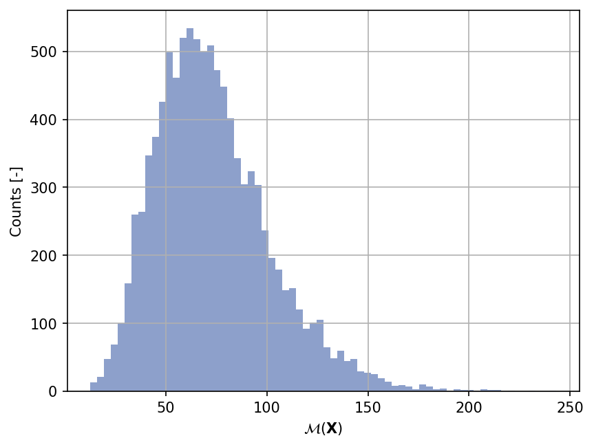
From the underlying probabilistic input model, a set of input values can be randomly generated. This is often useful for verification and validation purposes. For instance, to generate \(10'000\) sample points:
xx_sample = my_testfun.prob_input.get_sample(10000)
yy_sample = my_testfun(xx_sample)
The histogram of the output values can be created as follows:
Note
An ProbInput instance has a method called reset_rng();
You can call this method to create a new underlying RNG
perhaps with a seed number.
In that case, the seed number is optional; if not specified,
the system entropy is used to initialized
the NumPy default random generator.
In UQTestFuns, each instance of probabilistic input model carries its own pseudo-random number generator (RNG) to avoid using the global NumPy random RNG. See this blog post regarding some good practices on using NumPy RNG.
Transformation to the function domain#
Some UQ methods often produce sample points in a hypercube domain (for example, \([0, 1]^M\) or \([-1, 1]^M\) where \(M\) is the number of input dimension) at which the function should be evaluated. This hypercube domain may differ from the test function’s domain. Before the test function can be evaluated, those values must be first transformed to the function domain.
UQTestFuns provides a convenient function to transform sample points in one domain to the function domain. For instance, suppose we have a sample of size \(5\) in \([-1, 1]^8\) for the borehole function:
rng_1 = np.random.default_rng(42)
xx_sample_dom_1 = rng_1.uniform(low=-1, high=1, size=(5, 8))
xx_sample_dom_1
array([[ 0.5479121 , -0.12224312,  0.71719584,  0.39473606, -0.8116453 ,
         0.9512447 ,  0.5222794 ,  0.57212861],
       [-0.74377273, -0.09922812, -0.25840395,  0.85352998,  0.28773024,
         0.64552323, -0.1131716 , -0.54552256],
       [ 0.10916957, -0.87236549,  0.65526234,  0.2633288 ,  0.51617548,
        -0.29094806,  0.94139605,  0.78624224],
       [ 0.55676699, -0.61072258, -0.06655799, -0.91239247, -0.69142102,
         0.36609791,  0.48952431,  0.93501946],
       [-0.34834928, -0.25908059, -0.06088838, -0.62105728, -0.74015699,
        -0.04859015, -0.5461813 ,  0.33962799]])
We can transform this set of values to the domain of the function
via the transform_sample() method:
xx_sample_trans_1 = my_testfun.transform_sample(xx_sample_dom_1)
xx_sample_trans_1
array([[1.12167271e-01, 1.91089168e+03, 1.08172149e+05, 1.06671048e+03,
        6.80819817e+01, 8.17074682e+02, 1.54623823e+03, 1.16042925e+04],
       [8.16286191e-02, 1.96768976e+03, 8.25480202e+04, 1.09194415e+03,
        9.71604649e+01, 7.98731394e+02, 1.36831195e+03, 1.04531118e+04],
       [1.02220926e-01, 4.82013357e+02, 1.06545465e+05, 1.05948308e+03,
        1.03202841e+02, 7.42543116e+02, 1.66359089e+03, 1.18248295e+04],
       [1.12406858e-01, 9.38469433e+02, 8.75868543e+04, 9.94818414e+02,
        7.12619141e+01, 7.81965874e+02, 1.53706681e+03, 1.19780700e+04],
       [9.26946708e-02, 1.59960562e+03, 8.77357668e+04, 1.01084185e+03,
        6.99728476e+01, 7.57084591e+02, 1.24706924e+03, 1.13648168e+04]])
By default, the method assumes the uniform domain of the passed values is in \([-1, 1]^M\). It is possible to transform values defined in another uniform domain. For example, the sample values in \([0, 1]^8\) (a unit hypercube):
rng_2 = np.random.default_rng(42)
xx_sample_dom_2 = rng_2.random((5, 8))
xx_sample_dom_2
array([[0.77395605, 0.43887844, 0.85859792, 0.69736803, 0.09417735,
        0.97562235, 0.7611397 , 0.78606431],
       [0.12811363, 0.45038594, 0.37079802, 0.92676499, 0.64386512,
        0.82276161, 0.4434142 , 0.22723872],
       [0.55458479, 0.06381726, 0.82763117, 0.6316644 , 0.75808774,
        0.35452597, 0.97069802, 0.89312112],
       [0.7783835 , 0.19463871, 0.466721  , 0.04380377, 0.15428949,
        0.68304895, 0.74476216, 0.96750973],
       [0.32582536, 0.37045971, 0.46955581, 0.18947136, 0.12992151,
        0.47570493, 0.22690935, 0.66981399]])
can be transformed to the domain of the borehole function as follows:
xx_sample_trans_2 = my_testfun.transform_sample(
    xx_sample_dom_2, min_value=0.0, max_value=1.0
)
xx_sample_trans_2
array([[1.12167271e-01, 1.91089168e+03, 1.08172149e+05, 1.06671048e+03,
        6.80819817e+01, 8.17074682e+02, 1.54623823e+03, 1.16042925e+04],
       [8.16286191e-02, 1.96768976e+03, 8.25480202e+04, 1.09194415e+03,
        9.71604649e+01, 7.98731394e+02, 1.36831195e+03, 1.04531118e+04],
       [1.02220926e-01, 4.82013357e+02, 1.06545465e+05, 1.05948308e+03,
        1.03202841e+02, 7.42543116e+02, 1.66359089e+03, 1.18248295e+04],
       [1.12406858e-01, 9.38469433e+02, 8.75868543e+04, 9.94818414e+02,
        7.12619141e+01, 7.81965874e+02, 1.53706681e+03, 1.19780700e+04],
       [9.26946708e-02, 1.59960562e+03, 8.77357668e+04, 1.01084185e+03,
        6.99728476e+01, 7.57084591e+02, 1.24706924e+03, 1.13648168e+04]])
Note that for a given sample, the bounds of the hypercube domain must be the same in all dimensions.
The two transformed values above should be the same since we use two instances of the default RNG with the same seed to generate the random sample.
assert np.allclose(xx_sample_trans_1, xx_sample_trans_2)
assert np.allclose(my_testfun(xx_sample_trans_1), my_testfun(xx_sample_trans_2))
Test functions with parameters#
Some test functions are parameterized; this means that to fully specify the function, an additional set of values must be specified. In principle, these parameter values can be anything: numerical values, flags, selection using strings, etc.
For instance, consider the Ishigami function [IH91] defined as follows:
where \(a\) and \(b\) are the so-called parameters of the function.
Before the function can be evaluated,
these parameters must be assigned to some values.
The default Ishigami function in UQTestFuns has these values given
and stored in the parameters property:
my_testfun = uqtf.Ishigami()

print(my_testfun.parameters)
Function ID  : Ishigami
Parameter ID : Ishigami1991
Description  : Parameter set for the Ishigami function from Ishigami and
               Homma (1991)

 No.    Keyword      Value      Type    Description
-----  ---------  -----------  ------  -------------
  1        a      7.00000e+00  float
  2        b      1.00000e-01  float
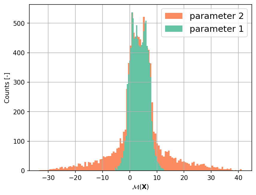
To assign different parameter values, override the property values of the instance by specifying the name in brackets just like a dictionary: For example:
my_testfun.parameters["a"] = 7.0
my_testfun.parameters["b"] = 0.35
Note that once set, the parameter values are kept constant during the evaluation of the function on a set of input values
Different parameter values usually change the overall behavior of the function. In the case of the Ishigami function, different parameter values alter the total variance of the output as illustrated in the figure below.
Test functions with variable dimension#
Some test functions support a variable dimension, meaning that an instance of a test function can be constructed for any number (positive integer, please) of input dimension.
Consider, for instance, the Sobol’-G function [SSobol95], a test function whose dimension can be varied and a popular choice in the context of sensitivity analysis. It is defined as follows:
where \(\boldsymbol{x} = \{ x_1, \ldots, x_M \}\) is the \(M\)-dimensional vector of input variables, and \(\boldsymbol{a} = \{ a_1, \ldots, a_M \}\) are parameters of the function.
To create a six-dimensional Sobol’-G function,
use the parameter input_dimension to specify the desired dimensionality:
my_testfun = uqtf.SobolG(input_dimension=6)
Verify that the function is indeed a six-dimension one:
print(my_testfun)
Function ID      : SobolG
Input Dimension  : 6 (variable)
Output Dimension : 1
Parameterized    : True
Description      : Sobol'-G function from Saltelli and Sobol' (1995)
Applications     : sensitivity, integration
and:
print(my_testfun.prob_input)
Function ID     : SobolG
Input ID        : Saltelli1995
Input Dimension : 6
Description     : Probabilistic input model for the Sobol'-G function from
                  Saltelli and Sobol' (1995)
Marginals       :

 No.    Name    Distribution    Parameters    Description
-----  ------  --------------  ------------  -------------
  1      X1       uniform        [0. 1.]           -
  2      X2       uniform        [0. 1.]           -
  3      X3       uniform        [0. 1.]           -
  4      X4       uniform        [0. 1.]           -
  5      X5       uniform        [0. 1.]           -
  6      X6       uniform        [0. 1.]           -

Copulas         : Independence
References#
William V. Harper and Sumant K. Gupta. Sensitivity/uncertainty analysis of a borehole scenario comparing latin hypercube sampling and deterministic sensitivity approaches. Technical Report BMI/ONWI-516, Office of Nuclear Waste Isolation, Battelle Memorial Institute, 1983. URL: https://inldigitallibrary.inl.gov/PRR/84393.pdf.
T. Ishigami and T. Homma. An importance quantification technique in uncertainty analysis for computer models. In [1990] Proceedings. First International Symposium on Uncertainty Modeling and Analysis, 398–403. IEEE Comput. Soc. Press, 1991. doi:10.1109/ISUMA.1990.151285.
Andrea Saltelli and Ilya M. Sobol'. About the use of rank transformation in sensitivity analysis of model output. Reliability Engineering & System Safety, 50(3):225–239, 1995. doi:10.1016/0951-8320(95)00099-2.