Test Functions for Reliability Analysis#
The table below listed the available test functions typically used in the comparison of reliability analysis methods.
Name |
Input Dimension |
Constructor |
|---|---|---|
2 |
|
|
2 |
|
|
2 |
|
|
8 |
|
|
2 |
|
|
2 |
|
|
2 |
|
|
2 |
|
|
2 |
|
|
5 |
|
|
6 |
|
In a Python terminal, you can list all the available functions relevant
for metamodeling applications using list_functions() and filter the results
using the tag parameter:
import uqtestfuns as uqtf

uqtf.list_functions(tag="reliability", tablefmt="html")
| No. | Constructor | # Input | # Output | Param. | Description |
|---|---|---|---|---|---|
| 1 | CantileverBeam2D() | 2 | 1 | True | Cantilever beam reliability problem from Rajashekhar and Ellington (1993) |
| 2 | CircularPipeCrack() | 2 | 1 | True | Circular pipe under bending moment from Verma et al. (2015) |
| 3 | ConvexFailDomain() | 2 | 1 | False | Convex failure domain problem from Borri and Speranzini (1997) |
| 4 | DampedOscillatorReliability() | 8 | 1 | True | Performance function from Der Kiureghian and De Stefano (1990) |
| 5 | FourBranch() | 2 | 1 | True | Series system reliability from Katsuki and Frangopol (1994) |
| 6 | GaytonHat() | 2 | 1 | False | Two-Dimensional Gayton Hat function from Echard et al. (2013) |
| 7 | HyperSphere() | 2 | 1 | False | Hyper-sphere bound reliability problem from Li et al. (2018) |
| 8 | RSCircularBar() | 2 | 1 | True | RS problem as a circular bar from Verma et al. (2016) |
| 9 | RSQuadratic() | 2 | 1 | False | RS problem w/ one quadratic term from Waarts (2000) |
| 10 | SpeedReducerShaft() | 5 | 1 | False | Reliability of a shaft in a speed reducer from Du and Sudjianto (2004) |
| 11 | UndampedOscillator() | 6 | 1 | False | Undamped, non-linear, single DOF oscillator |
About reliability analysis#
Consider a system whose performance is defined by a performance function[1] \(g\) whose values, in turn, depend on:
\(\boldsymbol{x}_p\): the (uncertain) input variables of the underlying computational model \(\mathcal{M}\)
\(\boldsymbol{x}_s\): additional (uncertain) input variables that affects the performance of the system, but not part of inputs to \(\mathcal{M}\)
\(\boldsymbol{p}\): an additional set of deterministic parameters of the system
Combining these variables and parameters as an input to the performance function \(g\):
where \(\boldsymbol{x} = \{ \boldsymbol{x}_p, \boldsymbol{x}_s \}\).
The system is said to be in failure state if and only if \(g(\boldsymbol{x}; \boldsymbol{p}) \leq 0\); the set of all values \(\{ \boldsymbol{x}, \boldsymbol{p} \}\) such that \(g(\boldsymbol{x}; \boldsymbol{p}) \leq 0\) is called the failure domain.
Conversely, the system is said to be in safe state if and only if \(g(\boldsymbol{x}; \boldsymbol{p}) > 0\); the set of all values \(\{ \boldsymbol{x}, \boldsymbol{p} \}\) such that \(g(\boldsymbol{x}; \boldsymbol{p}) > 0\) is called the safe domain.
Note
For example, taken in the context of nuclear engineering, a performance function may be defined for the fuel cladding temperature. The maximum temperature during a transient is computed using a computation model. A hypothetical regulatory limit of the maximum temperature is provided but with an uncertainty considering the variability in the high-temperature performance within the cladding population. The system is in failure state if the maximum temperature during a transient as computed by the model exceeds the regulatory limit; vice versa, the system is in safe state if the maximum temperature does not exceed the regulatory limit.
Reliability analysis[2] concerns with estimating the failure probability of a system with a given performance function \(g\). For a given joint probability density function (PDF) \(f_{\boldsymbol{X}}\) of the uncertain input variables \(\boldsymbol{X} = \{ \boldsymbol{X}_p, \boldsymbol{X}_s \}\), the failure probability \(P_f\) of the system is defined as follows [Sud12, VAK15]:
Evaluating the above integral is, in general, non-trivial because the domain of integration is only provided implicitly and the number of dimensions may be large.
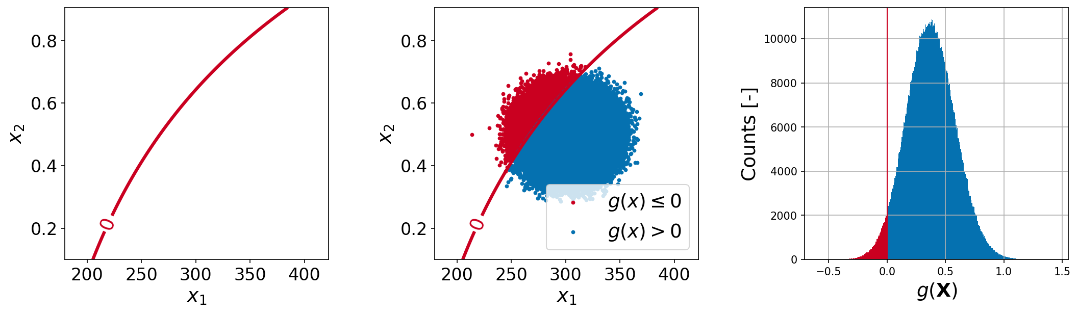
A series of plots below illustrates the reliability analysis problem in two dimensions. The left plot shows the limit-state surface (i.e., \(\boldsymbol{x}\) where \(g(\boldsymbol{x}) = 0\)) in the input parameter space. In the middle plot, \(10^6\) sample points are randomly generated and overlaid. The red points (resp. blue points) indicate that the points fall in the failure domain (resp. safe domain). Finally, the histogram on the right shows the failure probability, i.e., the area under the histogram such that \(g(\boldsymbol{x}) \leq 0\). The task of reliability analysis methods is to estimate the failure probability accurately with as few function/model evaluations as possible.
References#
Bruno Sudret. Meta-models for structural reliability and uncertainty quantification. In Proceedings of the 5th Asian-Pacific Symposium on Structural Reliability and its Applications. 2012. doi:10.3850/978-981-07-2219-7_p321.
Ajit Kumar Verma, Srividya Ajit, and Durga Rao Karanki. Structural reliability. In Springer Series in Reliability Engineering, pages 257–292. Springer London, 2015. doi:10.1007/978-1-4471-6269-8_8.