One-dimensional (1D) Damped Cosine Function

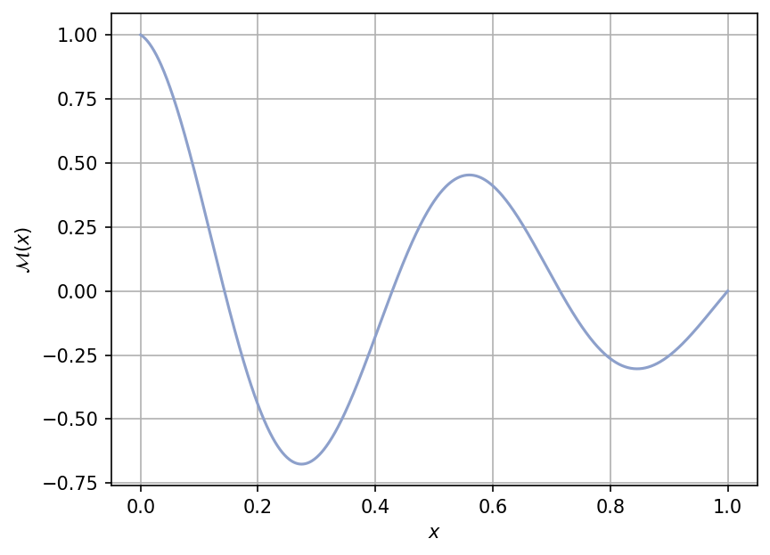
The 1D damped cosine function from Santner et al. [SWN18] is a scalar-valued test function for metamodeling exercises.

import numpy as np
import matplotlib.pyplot as plt
import uqtestfuns as uqtf

A plot of the function is shown below for \(x \in [0, 1]\).

Test function instance

To create a default instance of the test function:

my_testfun = uqtf.DampedCosine()

Check if it has been correctly instantiated:

print(my_testfun)

Function ID      : DampedCosine
Input Dimension  : 1 (fixed)
Output Dimension : 1
Parameterized    : False
Description      : One-dimensional damped cosine from Santner et al. (2018)
Applications     : metamodeling

Description

The test function is analytically defined as follows[1]:

\[ \mathcal{M}(x) = e^{(-1.4 x)} \cos{(3.5 \pi x)}, \]

where \(x\) is defined below.

Probabilistic input

Based on [SWN18], the domain of the function is in \([0, 1]\). In UQTestFuns, this domain can be represented as a probabilistic input model using the uniform distribution shown in the table below.

Show code cell source

Hide code cell source

print(my_testfun.prob_input)

Function ID     : DampedCosine
Input ID        : Santner2018
Input Dimension : 1
Description     : Input model for the one-dimensional damped cosine from
                  Santner et al. (2018)
Marginals       :

 No.    Name    Distribution    Parameters    Description
-----  ------  --------------  ------------  -------------
  1      x        uniform        [0. 1.]           -

Reference results

This section provides several reference results of typical UQ analyses involving the test function.

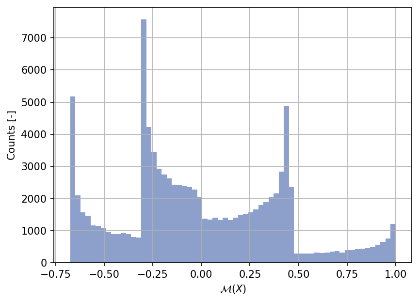
Sample histogram

Shown below is the histogram of the output based on \(100'000\) random points:

Show code cell source

Hide code cell source

np.random.seed(42)
xx_test = my_testfun.prob_input.get_sample(100000)
yy_test = my_testfun(xx_test)

plt.hist(yy_test, bins="auto", color="#8da0cb");
plt.grid();
plt.ylabel("Counts [-]");
plt.xlabel("$\mathcal{M}(X)$");
plt.gcf().tight_layout(pad=3.0)
plt.gcf().set_dpi(150);

Moment estimations

Shown below is the convergence of a direct Monte-Carlo estimation of the output mean and variance with increasing sample sizes.

Show code cell source

Hide code cell source

np.random.seed(42)
sample_sizes = np.array([1e1, 1e2, 1e3, 1e4, 1e5, 1e6], dtype=int)
mean_estimates = np.empty((len(sample_sizes), 50))
var_estimates = np.empty((len(sample_sizes), 50))

for i, sample_size in enumerate(sample_sizes):
    for j in range(50):
        xx_test = my_testfun.prob_input.get_sample(sample_size)
        yy_test = my_testfun(xx_test)
        mean_estimates[i, j] = np.mean(yy_test)
        var_estimates[i, j] = np.var(yy_test)

# --- Compute the error associated with the estimates
mean_estimates_errors = np.std(mean_estimates, axis=1)
var_estimates_errors = np.std(var_estimates, axis=1)

# --- Plot the mean and variance estimates
fig, ax_1 = plt.subplots(figsize=(6,4))

# --- Mean plot
ax_1.errorbar(
    sample_sizes,
    mean_estimates[:,0],
    yerr=2.0*mean_estimates_errors,
    marker="o",
    color="#66c2a5",
    label="Mean"
)
ax_1.set_xlim([5, 2e6])
ax_1.set_xlabel("Sample size")
ax_1.set_ylabel("Output mean estimate")
ax_1.set_xscale("log");
ax_2 = ax_1.twinx()

# --- Variance plot
ax_2.errorbar(
    sample_sizes+1,
    var_estimates[:,0],
    yerr=1.96*var_estimates_errors,
    marker="o",
    color="#fc8d62",
    label="Variance",
)
ax_2.set_ylabel("Output variance estimate")

# Add the two plots together to have a common legend
ln_1, labels_1 = ax_1.get_legend_handles_labels()
ln_2, labels_2 = ax_2.get_legend_handles_labels()
ax_2.legend(ln_1 + ln_2, labels_1 + labels_2, loc=0)

plt.grid()
fig.set_dpi(150)

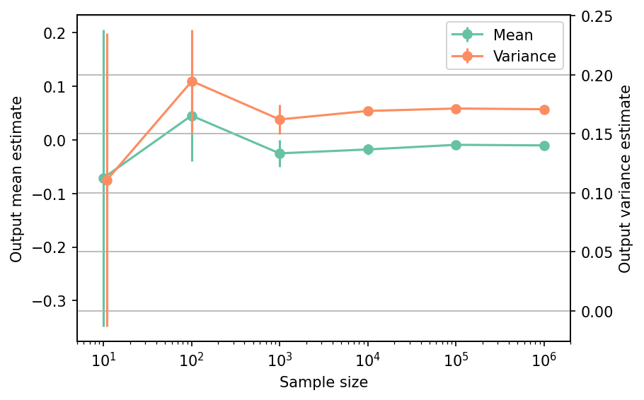
The tabulated results for each sample size is shown below.

Show code cell source

Hide code cell source

from tabulate import tabulate

# --- Compile data row-wise
outputs =[]

for (
    sample_size,
    mean_estimate,
    mean_estimate_error,
    var_estimate,
    var_estimate_error,
) in zip(
    sample_sizes,
    mean_estimates[:,0],
    2.0*mean_estimates_errors,
    var_estimates[:,0],
    2.0*var_estimates_errors,
):
    outputs += [
        [
            sample_size,
            mean_estimate,
            mean_estimate_error,
            var_estimate,
            var_estimate_error,
            "Monte-Carlo",
        ],
    ]

header_names = [
    "Sample size",
    "Mean",
    "Mean error",
    "Variance",
    "Variance error",
    "Remark",
]

tabulate(
    outputs,
    numalign="center",
    stralign="center",
    tablefmt="html",
    floatfmt=(".1e", ".4e", ".4e", ".4e", ".4e", "s"),
    headers=header_names
)

Sample size	Mean	Mean error	Variance	Variance error	Remark
10	-7.1324e-02	2.7675e-01	1.1090e-01	1.2665e-01	Monte-Carlo
100	4.5017e-02	8.5058e-02	1.9454e-01	4.4512e-02	Monte-Carlo
1000	-2.5314e-02	2.5099e-02	1.6208e-01	1.2621e-02	Monte-Carlo
10000	-1.8074e-02	9.6450e-03	1.6928e-01	3.8623e-03	Monte-Carlo
100000	-9.4371e-03	2.4299e-03	1.7134e-01	1.3109e-03	Monte-Carlo
1000000	-1.0507e-02	8.1401e-04	1.7073e-01	3.7487e-04	Monte-Carlo

References

[SWN18] (1,2,3)

Thomas J. Santner, Brian J. Williams, and William I. Notz. The design and analysis of computer experiments. Springer New York, 2018. doi:10.1007/978-1-4939-8847-1.

---

[1]

see Example 3.3 in [SWN18].