One-dimensional (1D) Forrester et al. (2008) Function

The 1D Forrester et al. (2008) function (or Forrester2008 function for short) is a one-dimensional scalar-valued function. It was used in [FSK08] as a test function for illustrating optimization using metamodels.

import numpy as np
import matplotlib.pyplot as plt
import uqtestfuns as uqtf

A plot of the function is shown below for \(x \in [0, 1]\).

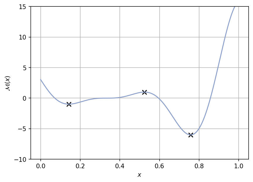
As can be seen in the plot above, the function features a multimodal shape with one global minimum (\(\approx -6.02074006\) at \(x = 0.75724876\)), one global maximum (\(\approx -0.98632541\) at \(x = 014258919\)), and an inflection point with zero gradient (\(\approx -6.02074006\) at \(x = 0.5240772\)).

Test function instance

To create a default instance of the test function:

my_testfun = uqtf.Forrester2008()

Check if it has been correctly instantiated:

print(my_testfun)

Name              : Forrester2008
Spatial dimension : 1
Description       : One-dimensional function from Forrester et al. (2008)

Description

The test function is analytically defined as follows:

\[ \mathcal{M}(x) = (6 x - 2)^2 \sin{(12 x - 4)}, \]

where \(x\) is defined below.

Input

Based on [FSK08], the search domain of the function is in \([0, 1]\). In UQTestFuns, this search domain can be represented as probabilistic input using the uniform distribution with a marginal shown in the table below.

my_testfun.prob_input

Name: Forrester2008

Spatial Dimension: 1

Description: Input specification for the 1D test function from Forrester et al. (2008)

Marginals:

No.	Name	Distribution	Parameters	Description
1	x	uniform	[0 1]	None

Copulas: None

Reference results

This section provides several reference results of typical UQ analyses involving the test function.

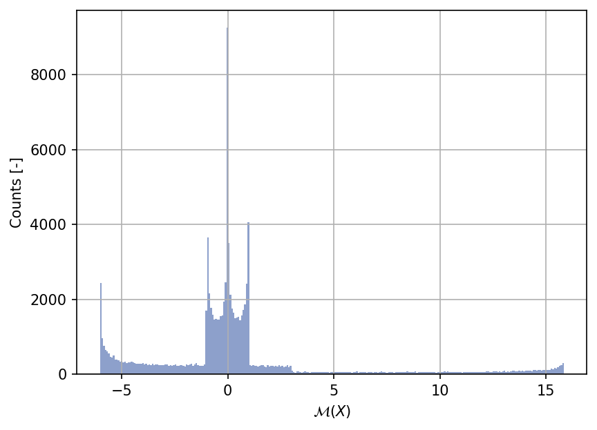
Sample histogram

Shown below is the histogram of the output based on \(100'000\) random points:

np.random.seed(42)
xx_test = my_testfun.prob_input.get_sample(100000)
yy_test = my_testfun(xx_test)

plt.hist(yy_test, bins="auto", color="#8da0cb");
plt.grid();
plt.ylabel("Counts [-]");
plt.xlabel("$\mathcal{M}(X)$");
plt.gcf().tight_layout(pad=3.0)
plt.gcf().set_dpi(150);

Optimum values

The optimum values of the function are:

• Global minimum: \(\mathcal{M}(\boldsymbol{x}^*) \approx -6.02074006\) at \(x^* = 0.75724876\).

• Local minimum: \(\mathcal{M}(\boldsymbol{x}^*) \approx -0.98632541\) at \(x^* = 014258919\).

• Inflection: \(\mathcal{M}(\boldsymbol{x}^*) \approx -6.02074006\) at \(x^* = 0.5240772\).

References

FSK08(1,2)

Alexander I. J. Forrester, András Sóbester, and Andy J. Keane. Engineering Design via Surrogate Modelling: A Practical Guide. Wiley, 1 edition, 2008. ISBN 978-0-470-06068-1 978-0-470-77080-1. doi:10.1002/9780470770801.