(1st) Franke Function#

import numpy as np
import matplotlib.pyplot as plt
import uqtestfuns as uqtf

The (1st) Franke function is a two-dimensional scalar-valued function. The function was first introduced in [Fra79] in the context of interpolation problem and was used in [HQ11] in the context of metamodeling.

Note

The Franke’s original report [Fra79] contains in total six two-dimensional test functions:

(1st) Franke function: Two Gaussian peaks and a Gaussian dip on a surface slopping down the upper right boundary (this function)
(2nd) Franke function: Two nearly flat regions joined by a sharp rise running diagonally
(3rd) Franke function: A saddle shaped surface
(4th) Franke function: A Gaussian hill that slopes off in a gentle fashion
(5th) Franke function: A steep Gaussian hill that approaches zero at the boundaries
(6th) Franke function: A part of a sphere

The term “Franke function” typically only refers to the (1st) Franke function.

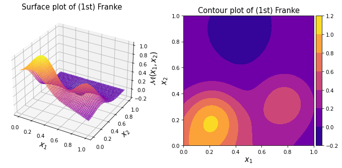
As shown in the plots above, the surface consists of two Gaussian peaks and a Gaussian dip on a surface sloping down toward the upper right boundary (i.e., at \((1.0, 1.0)\)).

Test function instance#

To create a default instance of the Franke function:

my_testfun = uqtf.Franke1()

Check if it has been correctly instantiated:

print(my_testfun)

Name              : Franke1
Spatial dimension : 2
Description       : (1st) Franke function from Franke (1979)

Description#

The Franke function is defined as follows:

\[\begin{split} \begin{align} \mathcal{M}(\boldsymbol{x}) = & 0.75 \exp{\left( -0.25 \left( (x_1 - 2)^2 + (x_2 - 2)^2 \right) \right) } \\ & + 0.75 \exp{\left( -1.00 \left( \frac{(x_1 + 1)^2}{49} + \frac{(x_2 + 1)^2}{10} \right) \right)} \\ & + 0.50 \exp{\left( -0.25 \left( (x_1 - 7)^2 + (x_2 - 3)^2 \right) \right)} \\ & - 0.20 \exp{\left( -1.00 \left( (x_1 - 4)^2 + (x_2 - 7)^2 \right) \right)} \\ \end{align} \end{split}\]

where \(\boldsymbol{x} = \{ x_1, x_2 \}\) is the two-dimensional vector of input variables further defined below.

Probabilistic input#

Based on [Fra79], the probabilistic input model for the function consists of two independent random variables as shown below.

my_testfun.prob_input

Name: Franke1979

Spatial Dimension: 2

Description: Input specification for the test functions from Franke (1979).

Marginals:

No.	Name	Distribution	Parameters	Description
1	X1	uniform	[0. 1.]	None
2	X2	uniform	[0. 1.]	None

Copulas: None

Reference results#

This section provides several reference results of typical UQ analyses involving the test function.

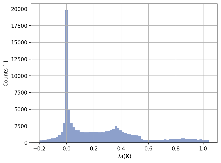
Sample histogram#

Shown below is the histogram of the output based on \(100'000\) random points:

xx_test = my_testfun.prob_input.get_sample(100000)
yy_test = my_testfun(xx_test)

plt.hist(yy_test, bins="auto", color="#8da0cb");
plt.grid();
plt.ylabel("Counts [-]");
plt.xlabel("$\mathcal{M}(\mathbf{X})$");
plt.gcf().set_dpi(150);

References#

Fra79(1,2,3): Richard Franke. A critical comparison of some methods for interpolation of scattered data. techreport NPS53-79-003, Naval Postgraduate School, Monterey, Canada, 1979. URL: https://core.ac.uk/reader/36727660.
HQ11: Ben Haaland and Peter Z. G. Qian. Accurate emulators for large-scale computer experiments. The Annals of Statistics, 39(6):2974–3002, 2011. doi:10.1214/11-aos929.

UQTestFuns

(1st) Franke Function

Contents