Four-branch Function#

import numpy as np
import matplotlib.pyplot as plt
import uqtestfuns as uqtf

The two-dimensional four-branch function was introduced in [KF94] and became a commonly used test function for reliability analysis algorithms (see, for instance, [SG05, Waa00, EGL11, SSM17]) The test function describes the failure of a series system with four distinct performance function components.

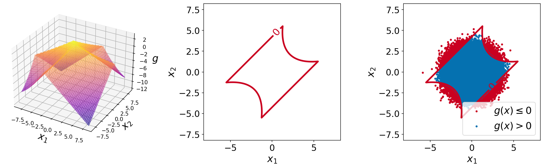
The plots of the function are shown below. The left plot shows the surface plot of the performance function, the center plot shows the contour plot with a single contour line at function value of \(0.0\) (the limit-state surface), and the right plot shows the same plot with \(10^6\) sample points overlaid.

Test function instance#

To create a default instance of the test function:

my_testfun = uqtf.FourBranch()

Check if it has been correctly instantiated:

print(my_testfun)

Name              : FourBranch
Spatial dimension : 2
Description       : Series system reliability from Katsuki and Frangopol (1994)

Description#

The test function (i.e., the performance function) is analytically defined as follows:

\[\begin{split} g(\boldsymbol{x}; p) = \min \begin{Bmatrix} 3 + 0.1 (x_1 - x_2)^2 - \frac{x_1 + x_2}{\sqrt{2}} \\ 3 + 0.1 (x_1 - x_2)^2 + \frac{x_1 + x_2}{\sqrt{2}} \\ (x_1 - x_2) + p \\ (x_2 - x_1) + p \\ \end{Bmatrix} \end{split}\]

where \(\boldsymbol{x} = \{ x_1, x_2 \}\) is the two-dimensional vector of input variables probabilistically defined further below and \(p\) is a deterministic parameter of the test function (see the corresponding section below).

The failure state and the failure probability are defined as \(g(\boldsymbol{x}; p) \leq 0\) and \(\mathbb{P}[g(\boldsymbol{X}; p) \leq 0]\), respectively.

Probabilistic input#

Based on [KF94], the probabilistic input model for the test function consists of two independent standard normal random variables (see the table below).

my_testfun.prob_input

Name: FourBranch-Katsuki1994

Spatial Dimension: 2

Description: Input model for the four-branch function from Katsuki and Frangopol (1994)

Marginals:

No.	Name	Distribution	Parameters	Description
1	X1	normal	[0 1]	None
2	X2	normal	[0 1]	None

Copulas: None

Parameters#

The test function is parameterized by a single value \(p\). Some values available in the literature is given in the table below.

\(p\)	Keyword	Source
\(3.5 \sqrt{2}\)	`Katsuki1994`	[KF94]
\(\frac{6}{\sqrt{2}}\)	`Schueremans2005` (default)	[SG05]

Reference results#

This section provides several reference results of typical UQ analyses involving the test function.

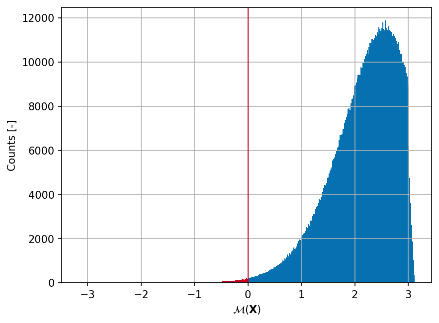
Sample histogram#

Shown below is the histogram of the output based on \(10^6\) random points:

xx_test = my_testfun.prob_input.get_sample(1000000)
yy_test = my_testfun(xx_test)
idx_pos = yy_test > 0
idx_neg = yy_test <= 0

hist_pos = plt.hist(yy_test, bins="auto", color="#0571b0")
plt.hist(yy_test[idx_neg], bins=hist_pos[1], color="#ca0020")
plt.axvline(0, linewidth=1.0, color="#ca0020")

plt.grid()
plt.ylabel("Counts [-]")
plt.xlabel("$\mathcal{M}(\mathbf{X})$")
plt.gcf().set_dpi(150);

Failure probability (\(P_f\))#

Some reference values for the failure probability \(P_f\) from the literature are summarized in the table below.

\(p\)	Method	\(N\)	\(\hat{P}_f\)	\(\mathrm{CoV}[\hat{P}_f]\)	Source
\(3.5 \sqrt{2}\)	Analytical	—	\(2.185961 \times 10^{-3}\)	—	[Waa00]
	MCS	\(10^5\)	\(2.185961 \times 10^{-3}\)	—	[Waa00]
	FORM	\(32\)	\(2.326291 \times 10^{-4}\)	—	[Waa00]
	SORM	\(12\)	\(8.740315 \times 10^{-4}\)	—	[Waa00]
\(\frac{6}{\sqrt{2}}\)	MCS	\(10^8\)	\(4.460 \times 10^{-3}\)	\(1.5 \%\)	[SSM17]
	MCS	\(10^6\)	\(4.416 \times 10^{-3}\)	\(0.15 \%\)	[EGL11]
	IS	\(1'469\)	\(4.9 \times 10^{-3}\)	—	[EGL11]

References#

SG05(1,2): Luc Schueremans and Dionys Van Gemert. Benefit of splines and neural networks in simulation based structural reliability analysis. Structural Safety, 27(3):246–261, 2005. doi:10.1016/j.strusafe.2004.11.001.
Waa00(1,2,3,4,5): Paul Hendrik Waarts. Structural reliability using finite element analysis - an appraisal of DARS: Directional adaptive response surface sampling. phdthesis, Civil Engineering and Geosciences, TU Delt, Delft, The Netherlands, 2000. URL: https://repository.tudelft.nl/islandora/object/uuid:6e6d9a76-fd12-4220-9dc1-36515b3f638d.
KF94(1,2,3): Satoshi Katsuki and Dan M. Frangopol. Hyperspace division method for structural reliability. Journal of Engineering Mechanics, 120(11):2405–2427, 1994. doi:10.1061/(asce)0733-9399(1994)120:11(2405).
EGL11(1,2,3): B. Echard, N. Gayton, and M. Lemaire. AK-MCS: an active learning reliability method combining kriging and Monte Carlo simulation. Structural Safety, 33(2):145–154, 2011. doi:10.1016/j.strusafe.2011.01.002.
SSM17(1,2): R. Schöbi, B. Sudret, and S. Marelli. Rare event estimation using polynomial-chaos kriging. ASCE-ASME Journal of Risk and Uncertainty in Engineering Systems, Part A: Civil Engineering, 2017. doi:10.1061/ajrua6.0000870.

UQTestFuns

Four-branch Function

Contents