Sulfur Model#
The sulfur model is a nine-dimensional scalar-valued function. Based on the model from [CSH+92], the model was used in [TPPM97] in the context of metamodeling and uncertainty propagation.
import numpy as np
import matplotlib.pyplot as plt
import uqtestfuns as uqtf
Test function instance#
To create a default instance of the sulfur model test function, type:
my_testfun = uqtf.Sulfur()
Check if the function has been correctly instantiated:
print(my_testfun)
Function ID      : Sulfur
Input Dimension  : 9 (fixed)
Output Dimension : 1
Parameterized    : False
Description      : Sulfur model from Charlson et al. (1992)
Applications     : metamodeling, sensitivity
Description#
The sulfur model analytically computes the direct radiative forcing by sulfate aerosols using the following expression:
where \(\boldsymbol{x} = \{ Q, Y, L, \Psi_e, \bar{\beta}, f_{\Psi_{e}}, T^2, (1 - A_c), (1 - R_s)^2 \}\) is the nine-dimensional vector of input variables further defined below.
To evaluate this expression, the values for two additional parameters are taken from the literature:
\(S_0 = 1361 \, [\mathrm{W/m^2}]\) (the solar constant) [KL11]
\(A = 5.1 \times 10^{14} \, [\mathrm{days}]\) (surface area of the earth) [Pid06]
Important
The equation for the sulfur model in [TPPM97] (Eq. (12)) is erroneous.
The solar constant \(S_0\) should not be squared otherwise the dimension will not agree.
The equation is missing factors 365 in the denominator and \(10^{12}\) in the numerator because the parameter \(L\) (sulfate lifetime in the atmosphere) is given in \([\mathrm{days}]\) while the parameter \(Q\) (global input flux of the anthropogenic sulfur) is given in \([\mathrm{T gS/year}]\)).
Probabilistic input#
The probabilistic input model for the sulfur model consists of nine independent uniform random variables with marginals shown in the table below. This specification is taken from [PCS+94] (Table 2); in the original specification, all parameters of the log-normal marginals are given in terms of geometric mean and geometric standard deviation.
Function ID     : Sulfur
Input ID        : Penner1994
Input Dimension : 9
Description     : Probabilistic input model for the Sulfur model from
                  Penner et al. (1994).
Marginals       :

 No.     Name     Distribution          Parameters                                             Description
-----  --------  --------------  -------------------------  ----------------------------------------------------------------------------------
  1       Q        lognormal      [4.26267988 0.13976194]                 Source strength of anthropogenic Sulfur [10^12 g/year]
  2       Y        lognormal     [-0.69314718  0.40546511]                   Fraction of SO2 oxidized to SO4(2-) aerosol [-]
  3       L        lognormal      [1.70474809 0.40546511]                     Average lifetime of atmospheric SO4(2-) [days]
  4     Psi_e      lognormal      [1.60943791 0.33647224]                       Aerosol mass scattering efficiency [m^2/g]
  5      beta      lognormal     [-1.2039728   0.26236426]                  Fraction of light scattered upward hemisphere [-]
  6    f_Psi_e     lognormal      [0.53062825 0.18232156]   Fractional increase in aerosol scattering efficiency due to hygroscopic growth [-]
  7      T^2       lognormal     [-0.54472718  0.33647224]             Square of atmospheric transmittance above aerosol layer [-]
  8     (1-Ac)     lognormal     [-0.94160854  0.09531018]                      Fraction of earth not covered by cloud [-]
  9    (1-Rs)^2    lognormal     [-0.32850407  0.18232156]                            Square of surface coalbedo [-]

Copulas         : Independence
Note
The geometric mean and the geometric standard deviation of a lognormal distribution are the exponentiated mu and sigma parameters (that is, the mean and the standard deviation of the underlying normal distribution), respectively.
While the probabilistic input specification in [TPPM97] is similar to the one in [PCS+94], the parameters \(T\) and \((1 - R_s)\) in [PCS+94] were given in the squared form (that is, \(T^2\) and \(1 - R_s)^2\)). This makes the formula simpler as it takes multiplicative form.
Reference results#
This section provides several reference results of typical UQ analyses involving the test function.
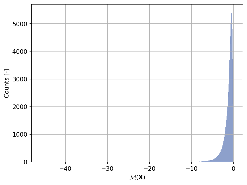
Sample histogram#
Shown below is the histogram of the output based on \(100'000\) random points:
Moments estimation#
Due to the multiplicative form of the function, the geometric mean (the mode) and the geometric standard deviation of the response are analytically available given the input specification (from [PCS+94], all input variables are log-normally distributed). The geometric mean is given as follows:
where \(\mu_{g, X_i}\)’s are the geometric mean of the input variables. Notice that all the (log) constants that appear in the equation must be added.
The geometric standard deviation is given as follows:
where \(\sigma_{g, X_i}\)’s are the geometric standard deviation of the input variables. The geometric variance of the output is then:
Shown below is the convergence of a direct Monte-Carlo estimation of the output mean and variance with increasing sample sizes compared with the analytical values. The error bars correspond to twice the standard deviation of the estimates obtained from \(25\) replications.
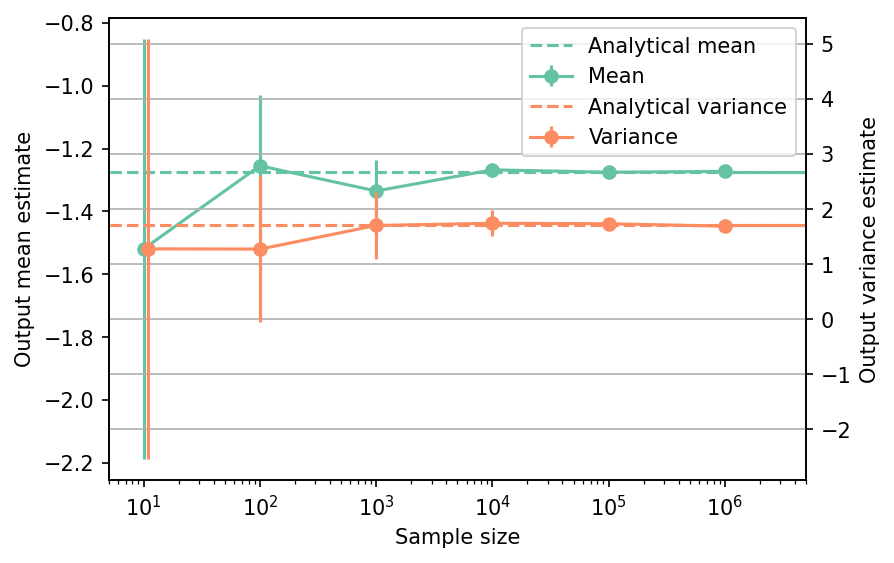
The tabulated results for is shown below.
| Sample size | Mean | Mean error | Variance | Variance error | Remark |
|---|---|---|---|---|---|
| nan | -1.2741 | 0.0000e+00 | 1.7089 | 0.0000e+00 | Analytical |
| 1.0e+01 | -1.5191 | 6.6762e-01 | 1.2794 | 3.8157e+00 | Monte-Carlo |
| 1.0e+02 | -1.2549 | 2.2633e-01 | 1.2764 | 1.3283e+00 | Monte-Carlo |
| 1.0e+03 | -1.3351 | 9.8148e-02 | 1.7046 | 6.1105e-01 | Monte-Carlo |
| 1.0e+04 | -1.2677 | 2.3202e-02 | 1.7452 | 2.3753e-01 | Monte-Carlo |
| 1.0e+05 | -1.2753 | 1.0202e-02 | 1.7362 | 7.5158e-02 | Monte-Carlo |
| 1.0e+06 | -1.2727 | 2.2953e-03 | 1.6917 | 1.9505e-02 | Monte-Carlo |
The convergence of a direct Monte-Carlo estimation of the output geometric mean and variance is shown below. As before the error bars are obtained by replicating the estimation.
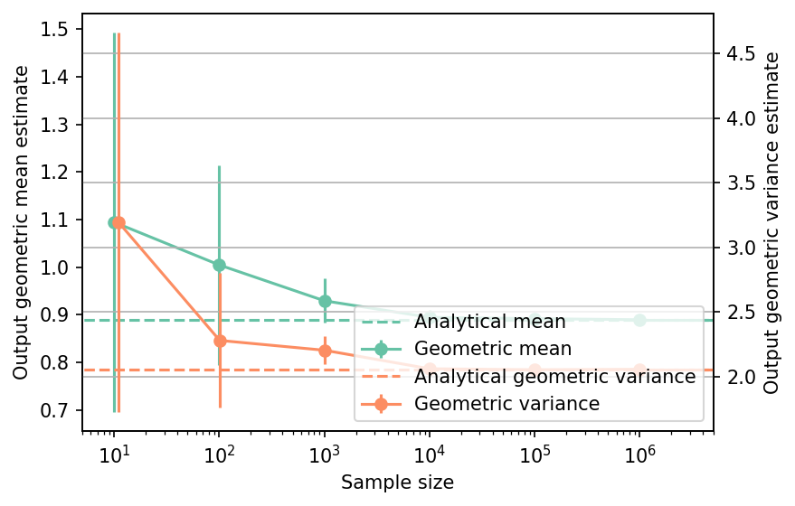
The corresponding tabulated results for is shown below.
| Sample size | Geom. mean | Geom. mean error | Geom. variance | Geom. variance error | Remark |
|---|---|---|---|---|---|
| nan | 8.8929e-01 | 0.0000e+00 | 2.0527 | 0.0000e+00 | Analytical |
| 1.0e+01 | 1.0944e+00 | 3.9870e-01 | 3.1938 | 1.4688e+00 | Monte-Carlo |
| 1.0e+02 | 1.0045e+00 | 2.0975e-01 | 2.2784 | 5.2250e-01 | Monte-Carlo |
| 1.0e+03 | 9.2923e-01 | 4.6337e-02 | 2.2024 | 1.0980e-01 | Monte-Carlo |
| 1.0e+04 | 8.9445e-01 | 1.5255e-02 | 2.0592 | 4.4181e-02 | Monte-Carlo |
| 1.0e+05 | 8.9176e-01 | 5.9974e-03 | 2.0514 | 1.2780e-02 | Monte-Carlo |
| 1.0e+06 | 8.8938e-01 | 1.5438e-03 | 2.0552 | 3.0666e-03 | Monte-Carlo |
References#
R. J. Charlson, S. E. Schwartz, J. M. Hales, R. D. Cess, J. A. Coakley, J. E. Hansen, and D. J. Hofmann. Climate forcing by anthropogenic aerosols. Science, 255(5043):423–430, 1992. doi:10.1126/science.255.5043.423.
Menner A. Tatang, Wenwei Pan, Ronald G. Prinn, and Gregory J. McRae. An efficient method for parametric uncertainty analysis of numerical geophysical models. Journal of Geophysical Research: Atmospheres, 102(D18):21925–21932, 1997. doi:10.1029/97jd01654.
Greg Kopp and Judith L. Lean. A new, lower value of total solar irradiance: evidence and climate significance. Geophysical Research Letters, 2011. doi:10.1029/2010gl045777.
M. Pidwirny. Fundamentals of Physical Geography, 2nd Edition, chapter Introduction to the oceans. Michael Pidwirny, 2006. URL: http://www.physicalgeography.net/fundamentals/8o.html.
J. E. Penner, R. J. Charlson, S. E. Schwartz, J. M. Hales, N. S. Laulainen, L. Travis, R. Leifer, T. Novakov, J. Ogren, and L. F. Radke. Quantifying and minimizing uncertainty of climate forcing by anthropogenic aerosols. Bulletin of the American Meteorological Society, 75(3):375–400, 1994. doi:10.1175/1520-0477(1994)075<0375:qamuoc>2.0.co;2.