Wing Weight Function#
import numpy as np
import matplotlib.pyplot as plt
import uqtestfuns as uqtf
The Wing Weight test function [FSK08] is a 10-dimensional scalar-valued function. The function has been used as a test function in the context of metamodeling [ZZP+20] and optimization [FSK08].
Test function instance#
To create a default instance of the wing weight test function:
my_testfun = uqtf.WingWeight()
Check if it has been correctly instantiated:
print(my_testfun)
Function ID      : WingWeight
Input Dimension  : 10 (fixed)
Output Dimension : 1
Parameterized    : False
Description      : Wing weight model from Forrester et al. (2008)
Applications     : metamodeling, sensitivity
Description#
The weight of a light aircraft wing is computed using the following analytical expression:
where \(\boldsymbol{x} = \{ S_w, W_{fw}, A, \Lambda, q, \lambda, t_c, N_z, W_{dg}, W_p\}\) is the vector of input variables defined below.
Probabilistic input#
Based on [FSK08], the probabilistic input model for the Wing Weight function consists of eight independent uniform random variables with ranges shown in the table below.
Function ID     : WingWeight
Input ID        : Forrester2008
Input Dimension : 10
Description     : Probabilistic input model for the Wing Weight model from
                  Forrester et al. (2008).
Marginals       :

 No.    Name    Distribution    Parameters                 Description
-----  ------  --------------  -------------  -------------------------------------
  1      Sw       uniform       [150. 200.]             wing area [ft^2]
  2     Wfw       uniform       [220. 300.]      weight of fuel in the wing [lb]
  3      A        uniform        [ 6. 10.]              aspect ratio [-]
  4    Lambda     uniform       [-10.  10.]       quarter-chord sweep [degrees]
  5      q        uniform        [16. 45.]    dynamic pressure at cruise [lb/ft^2]
  6    lambda     uniform        [0.5 1. ]               taper ratio [-]
  7      tc       uniform       [0.08 0.18]   aerofoil thickness to chord ratio [-]
  8      Nz       uniform        [2.5 6. ]          ultimate load factor [-]
  9     Wdg       uniform       [1700 2500]      flight design gross weight [lb]
 10      Wp       uniform      [0.025 0.08 ]         paint weight [lb/ft^2]

Copulas         : Independence
Reference Results#
This section provides several reference results of typical UQ analyses involving the test function.
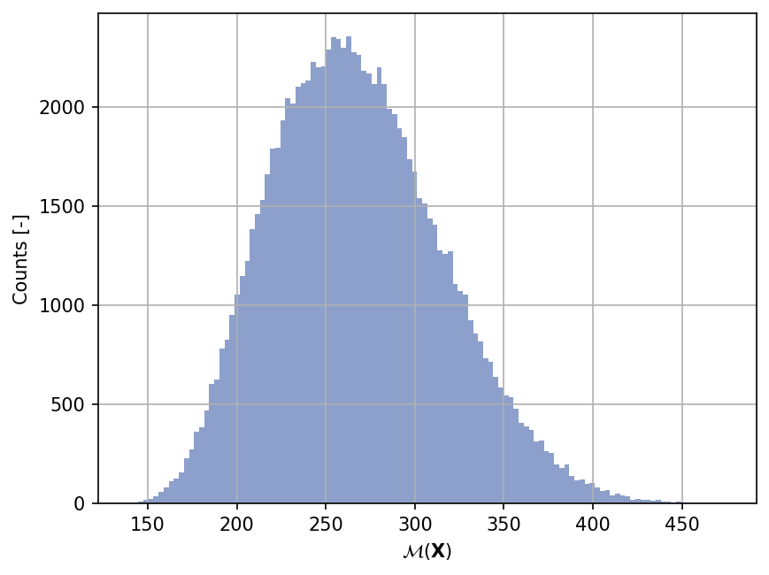
Sample histogram#
Shown below is the histogram of the output based on \(100'000\) random points:
Moments estimation#
Shown below is the convergence of a direct Monte-Carlo estimation of the output mean and variance with increasing sample sizes.

The tabulated results for each sample size is shown below.
| Sample size | Mean | Mean error | Variance | Variance error | Remark |
|---|---|---|---|---|---|
| 10 | 2.6046e+02 | 8.6249e+00 | 7.4389e+02 | 3.5067e+02 | Monte-Carlo |
| 100 | 2.6215e+02 | 4.8620e+00 | 2.3639e+03 | 3.3599e+02 | Monte-Carlo |
| 1000 | 2.6944e+02 | 1.5739e+00 | 2.4772e+03 | 1.1084e+02 | Monte-Carlo |
| 10000 | 2.6822e+02 | 4.8051e-01 | 2.3089e+03 | 3.2654e+01 | Monte-Carlo |
| 100000 | 2.6814e+02 | 1.5191e-01 | 2.3077e+03 | 1.0321e+01 | Monte-Carlo |
| 1000000 | 2.6815e+02 | 4.8135e-02 | 2.3170e+03 | 3.2768e+00 | Monte-Carlo |
| 10000000 | 2.6808e+02 | 1.5199e-02 | 2.3100e+03 | 1.0330e+00 | Monte-Carlo |
References#
Alexander I. J. Forrester, András Sóbester, and Andy J. Keane. Engineering Design via Surrogate Modelling: A Practical Guide. Wiley, 1 edition, 2008. ISBN 978-0-470-06068-1 978-0-470-77080-1. doi:10.1002/9780470770801.
Lavi R. Zuhal, Kemas Zakaria, Pramudita S. Palar, Koji Shimoyama, and Rhea P. Liem. Gradient-enhanced universal Kriging with polynomial chaos as trend function. In AIAA Scitech 2020 Forum. Orlando, Florida, 2020. American Institute of Aeronautics and Astronautics. doi:10.2514/6.2020-1865.