Piston Simulation Function#
import numpy as np
import matplotlib.pyplot as plt
import uqtestfuns as uqtf
The Piston simulation test function is a seven-dimensional scalar-valued function. The function computes the cycle time of a piston system.
This function has been used as a test function in metamodeling exercises [BAS07]. A 20-dimensional variant was used in the context of sensitivity analysis [Moo10] by introducing 13 additional inert input variables.
Test function instance#
To create a default instance of the piston simulation test function:
my_testfun = uqtf.Piston()
Check if it has been correctly instantiated:
print(my_testfun)
Function ID      : Piston
Input Dimension  : 7 (fixed)
Output Dimension : 1
Parameterized    : False
Description      : Piston simulation model from Ben-Ari and Steinberg (2007)
Applications     : metamodeling, sensitivity
Description#
The Piston simulation computes the cycle time of a piston moving inside a cylinder using the following analytical expression:
where \(\boldsymbol{x} = \{ M, S, V_0, k, P_0, T_a, T_0 \}\) is the seven-dimensional vector of input variables further defined below.
Probabilistic input#
Two probabilistic input model specifications for the OTL circuit function are available as shown in the table below.
The default selection, based on [BAS07], contains seven input variables given as independent uniform random variables with specified ranges shown in the table below.
Function ID     : Piston
Input ID        : BenAri2007
Input Dimension : 7
Description     : Probabilistic input model for the Piston simulation model
                  from Ben-Ari and Steinberg (2007).
Marginals       :

 No.    Name    Distribution      Parameters              Description
-----  ------  --------------  -----------------  ----------------------------
  1      M        uniform          [30. 60.]           Piston weight [kg]
  2      S        uniform        [0.005 0.02 ]     Piston surface area [m^2]
  3      V0       uniform        [0.002 0.01 ]      Initial gas volume [m^3]
  4      k        uniform        [1000. 5000.]      Spring coefficient [N/m]
  5      P0       uniform      [ 90000. 110000.]  Atmospheric pressure [N/m^2]
  6      Ta       uniform         [290. 296.]       Ambient temperature [K]
  7      T0       uniform         [340. 360.]     Filling gas temperature [K]

Copulas         : Independence
Note
In [Moo10], 13 additional inert independent input variables are introduced (totaling 20 input variables); these input variables, being inert, do not affect the output of the function.
To create an instance of the piston simulation test function
with the probabilistic input specified in [Moo10],
pass the corresponding keyword ("Moon2010")
to the parameter input_id):
my_testfun = uqtf.Piston(input_id="Moon2010")
Reference results#
This section provides several reference results of typical UQ analyses involving the test function.
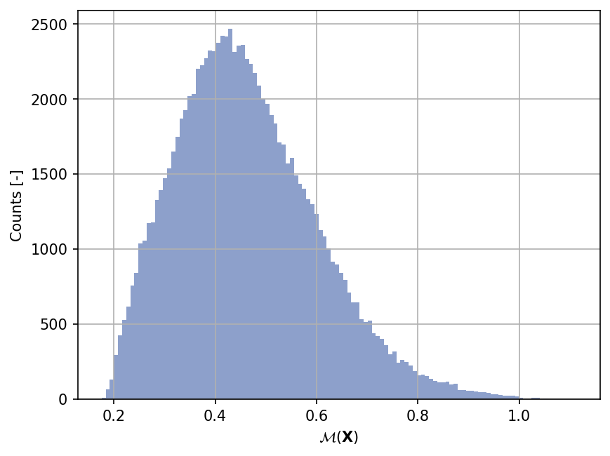
Sample histogram#
Shown below is the histogram of the output based on \(100'000\) random points:
Moments estimation#
Shown below is the convergence of a direct Monte-Carlo estimation of the output mean and variance with increasing sample sizes.
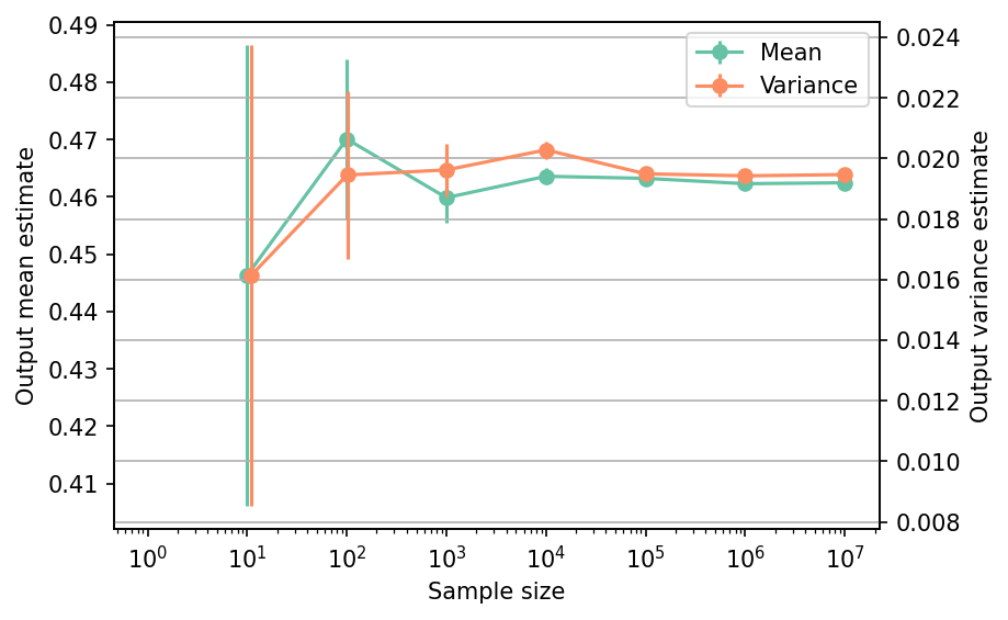
The tabulated results for each sample size is shown below.
| Sample size | Mean | Mean error | Variance | Variance error | Remark |
|---|---|---|---|---|---|
| 10 | 4.4632e-01 | 4.0173e-02 | 1.6139e-02 | 7.6080e-03 | Monte-Carlo |
| 100 | 4.7007e-01 | 1.3947e-02 | 1.9452e-02 | 2.7647e-03 | Monte-Carlo |
| 1000 | 4.5986e-01 | 4.4292e-03 | 1.9618e-02 | 8.7778e-04 | Monte-Carlo |
| 10000 | 4.6358e-01 | 1.4241e-03 | 2.0280e-02 | 2.8681e-04 | Monte-Carlo |
| 100000 | 4.6322e-01 | 4.4147e-04 | 1.9490e-02 | 8.7161e-05 | Monte-Carlo |
| 1000000 | 4.6229e-01 | 1.3937e-04 | 1.9424e-02 | 2.7469e-05 | Monte-Carlo |
| 10000000 | 4.6246e-01 | 4.4119e-05 | 1.9465e-02 | 8.7049e-06 | Monte-Carlo |
References#
Hyejung Moon. Design and analysis of computer experiments for screening input variables. PhD thesis, Ohio State University, Ohio, 2010. URL: http://rave.ohiolink.edu/etdc/view?acc_num=osu1275422248.
Einat Neumann Ben-Ari and David M. Steinberg. Modeling data from computer experiments: an empirical comparison of kriging with MARS and projection pursuit regression. Quality Engineering, 19(4):327–338, 2007. doi:10.1080/08982110701580930.