Simple Portfolio Model#
import numpy as np
import matplotlib.pyplot as plt
import uqtestfuns as uqtf
The simple portfolio model (or Portfolio3D for short ) is a three-dimensional
scalar-valued test function.
The function was introduced in [STCR04] as an example for
illustrating some elementary sensitivity measures.
Test function instance#
To create a default instance of the simple portfolio model:
my_testfun = uqtf.Portfolio3D()
Check if it has been correctly instantiated:
print(my_testfun)
Function ID      : Portfolio3D
Input Dimension  : 3 (fixed)
Output Dimension : 1
Parameterized    : True
Description      : Simple portfolio model from Saltelli et al. (2004)
Applications     : sensitivity
Description#
The simple portfolio model computes the estimated risk (return) in € of an investment portfolio consisting of three hedged portfolios via a linear relationship[1]:
where \(\boldsymbol{x} = \{ P_s, P_t, P_j \}\) is the vector of hedged portfolios values in € and \(\boldsymbol{p} = \{ C_s, C_t, C_j \}\) is the vector of quantities per hedged portfolio defined further below. \(\boldsymbol{x}\) is assumed to be random variables further defined below.
Probabilistic input#
Based on [STCR04], the probabilistic input model for the simple portfolio model consists of three independent normal random variables with the distribution parameters shown in the table below.
Function ID     : Portfolio3D
Input ID        : Saltelli2004
Input Dimension : 3
Description     : Probabilistic input model for the simple portfolio model
                  from Saltelli et al. (2004).
Marginals       :

 No.    Name    Distribution    Parameters         Description
-----  ------  --------------  ------------  ------------------------
  1      Ps        normal        [0. 4.]     Hedged portfolio 's' [€]
  2      Pt        normal        [0. 2.]     Hedged portfolio 't' [€]
  3      Pj        normal        [0. 1.]     Hedged portfolio 'j' [€]

Copulas         : Independence
Parameters#
The parameters of the simple portfolio model are the quantities of each of the hedged portfolios. The available values taken from [STCR04] are shown in the table below
No. |
Value |
Keyword |
Source |
|---|---|---|---|
1 |
\(C_s = 100\), \(C_t = 500\), \(C_j = 1000\) |
|
Table 1.1 [STCR04] |
2 |
\(C_s = 300\), \(C_t = 300\), \(C_j = 300\) |
|
Table 1.1 [STCR04] |
3 |
\(C_s = 500\), \(C_t = 400\), \(C_j = 100\) |
|
Table 1.1 [STCR04] |
The default value is shown below.
Function ID  : Portfolio3D
Parameter ID : Saltelli2004-1
Description  : Parameter set for the simple 3D portfolio model from
               Saltelli et al. (2004); the least volatile hedged
               portfolio is the largest quantity

 No.    Keyword      Value      Type             Description
-----  ---------  -----------  ------  -------------------------------
  1       cs      1.00000e+02  float   Quantities of the portfolio 's'
  2       ct      5.00000e+02  float   Quantities of the portfolio 't'
  3       cj      1.00000e+03  float   Quantities of the portfolio 'j'
Note
To create an instance of the simple portfolio model with a different set of parameter values from the selection above, type:
my_testfun = uqtf.Portfolio3D(parameters_id="Saltelli2004-2")
Reference results#
This section provides several reference results of typical UQ analyses involving the test function.
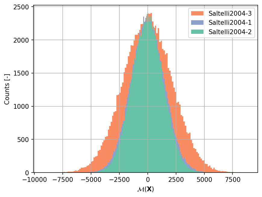
Sample histogram#
Shown below are the histograms of the output based on \(100'000\) random points for the simple portfolio model with three different sets of parameters.
Moments#
Based on the model structure as well as the assumption on the uncertain input variables, the output of the simple portfolio model is normally distributed. The moments are available analytically.
The mean reads:
where \(\bar{p}_s\), \(\bar{p}_t\), and \(\bar{p}_j\) are the means of the three hedged portfolios, respectively.
The standard deviation reads:
where \(\sigma_s\), \(\sigma_t\), and \(\sigma_j\) are the standard deviations of the three hedged portfolios, respectively.
The analytical values of the mean and standard deviation of the model output for the three sets of parameters are shown in the table below.
No. |
Parameter |
\(\bar{Y}\) |
\(\sigma_Y\) |
|---|---|---|---|
1 |
|
\(0.0\) |
\(1.4696938457 \times 10^3\) |
2 |
|
\(0.0\) |
\(1.3747727085 \times 10^3\) |
3 |
|
\(0.0\) |
\(2.1563858653 \times 10^3\) |
Sensitivity analysis#
In [STCR04], the simple portfolio model was used as an illustrating example of several model sensitivity measures. Due to the simple nature of the model (linear, monotonic), simple local or hybrid local-global sensitivity measures are deemed sufficient to characterize the model sensitivity.
Local sensitivity measure based derivative is given by:
This measure is dimensioned, but it happens that the dimension cancels out because the input \(P_x\) and the output \(Y\) have the same unit. The table below provides the analytical values of the local sensitivity measure for the three set of parameters.
Parameter |
\(P_s\) |
\(P_t\) |
\(P_j\) |
|---|---|---|---|
|
\(100\) |
\(500\) |
\(1'000\) |
|
\(300\) |
\(300\) |
\(300\) |
|
\(500\) |
\(400\) |
\(100\) |
To include the uncertainty of the input variables in the sensitivity measure, the local measure defined above is normalized by the standard deviation of both the input and the output. The hybrid local-global measure now reads:
The table below provides the analytical values of the sensitivity measure for the three different sets of parameters.
Parameter |
\(P_s\) |
\(P_t\) |
\(P_j\) |
|---|---|---|---|
|
\(0.272\) |
\(0.680\) |
\(0.680\) |
|
\(0.873\) |
\(0.436\) |
\(0.218\) |
|
\(0.928\) |
\(0.371\) |
\(0.046\) |
The measure \(S^{\sigma}_x\) has the following relation:
The relation implies that the main-effect Sobol’ sensitivity indices are the squared of the hybrid local-global measures.
Parameter |
\(P_s\) |
\(P_t\) |
\(P_j\) |
|---|---|---|---|
|
\(0.074\) |
\(0.4624\) |
\(0.4624\) |
|
\(0.762\) |
\(0.1900\) |
\(0.0475\) |
|
\(0.861\) |
\(0.1376\) |
\(0.0021\) |